<?xml version="1.0" encoding="utf-8"?><feed xmlns="http://www.w3.org/2005/Atom" ><generator uri="https://jekyllrb.com/" version="3.10.0">Jekyll</generator><link href="https://danylaksono.is-a.dev/feed.xml" rel="self" type="application/atom+xml" /><link href="https://danylaksono.is-a.dev/" rel="alternate" type="text/html" /><updated>2026-08-16T19:05:00-05:00</updated><id>https://danylaksono.is-a.dev/feed.xml</id><title type="html">Dany Laksono</title><subtitle>Geoinformatician</subtitle><author><name>Dany Laksono</name><email>dany.laksono@city.ac.uk</email></author><entry><title type="html">There is as Yet Insufficient Data for a Meaningful Answer</title><link href="https://danylaksono.is-a.dev/posts/2022/07/insufficient-data" rel="alternate" type="text/html" title="There is as Yet Insufficient Data for a Meaningful Answer" /><published>2022-07-05T00:00:00-05:00</published><updated>2022-07-05T00:00:00-05:00</updated><id>https://danylaksono.is-a.dev/posts/2022/07/insufficient-data</id><content type="html" xml:base="https://danylaksono.is-a.dev/posts/2022/07/insufficient-data"><![CDATA[<p>Since taking a job as a data scientist three months ago, I’ve spoken with multiple political science PhD students who are interested in potentially making the same transition. This post synthesizes what I’ve said in those conversations with what I’ve learned in my first three months on the job, and I hope it will be helpful to anyone in the same position I was six months ago.</p>

<!--more-->

<p>As I mentioned in my <a href="/posts/2022/03/so-it-goes">previous post</a>, I’m drawing inferences from an <em>n</em> of one, so take anything I say with a hefty grain of salt.<sup id="fnref:time" role="doc-noteref"><a href="#fn:time" class="footnote" rel="footnote">1</a></sup> While I’m structuring this post largely as pieces of advice, keep in mind that these were things that worked for me, and may not generalize.<sup id="fnref:negotiation" role="doc-noteref"><a href="#fn:negotiation" class="footnote" rel="footnote">2</a></sup></p>

<h1 id="differences-from-the-academic-job-market">Differences from the academic job market</h1>

<p>Some important differences between the academic and nonacademic job markets that are useful to consider at the start:</p>

<ul>
  <li>Timelines are faster than faculty searches, but they are far less consistent. One process took almost three months, while another took less than three weeks.</li>
  <li>Not a single employer asked for letters of recommendation. One contacted references.</li>
  <li>Who you talk to varies greatly. For some positions my first contact was an HR phone screen, for others it was a 30 minute initial interview with the hiring manager.</li>
  <li>Performance tasks, otherwise known as coding assignments (or, more accurately, unpaid work), are common. These are just a fact of life for data science jobs. They varied from straightforward problem sets to research design memos, but not every job I interviewed for required them.</li>
  <li>There will probably be a technical interview. As these were not software engineering jobs, most of the ones I encountered tried to assess whether you know the basics of analyzing data in your language of choice and to get some insight into your problem solving approaches.</li>
  <li>Job talks are much less common, but not unheard of. Only two of the positions I interviewed for required a technical presentation, and unlike in academia, there is absolutely zero stigma against presenting coauthored work.</li>
  <li>Based on some very informal reckoning, automated HR rejection emails seem to be about as common for nonacademic jobs as academic ones.<sup id="fnref:rejections" role="doc-noteref"><a href="#fn:rejections" class="footnote" rel="footnote">3</a></sup> When they do come, these emails are much faster than in academia: days or weeks instead of months.</li>
  <li>Get ready for a new world of terminology and titles. In the same way that the assistant $\rightarrow$ associate $\rightarrow$ full professor progression baffles many outside of academia, I felt very lost upon encountering ads for senior, principal, and lead data scientists, and especially so when I applied to one for a data science technical adviser.</li>
  <li>Similarly, get ready to navigate the variety of different jobs that can fall under the umbrella of data scientist. Does a job list SQL, Tableau, and Excel as the most important technical skills? That’s probably more of a data analyst position. TensorFlow, Dask, and C++? That’s likely more of machine learning engineer job. If you’re anything like me, you want to aim for the middle ground between these two.</li>
</ul>

<h1 id="the-nonacademic-résumé">The nonacademic résumé</h1>

<p>Probably the biggest transition when starting to apply for data science jobs was the shift from an academic CV to a nonacademic résumé. A CV lists functionally every major accomplishment you’ve achieved in your time in the field, while a résumé is highly targeted for a specific position. When applying to academic jobs, I wrote a (semi) customized cover letter for every job, and then included the relevant version of my CV (conflict, methods, or teaching). Each of these CVs contained the same information, just in a different order. In contrast, I significantly edited the skills section of most résumés I sent out based on the job listing. The <a href="https://students.wustl.edu/career-center">WashU career center</a> has a <a href="https://students.wustl.edu/wp-content/uploads/2021/02/Resumes-and-CVs-2021-Final-1.pdf">fantastic handout</a> on differences between the two documents and how to adapt a CV into a résumé that I drew on heavily in this process.</p>

<p>In my opinion, the conventional wisdom that a résumé can only ever be one page is an overcorrection from the never-ending academic CV. The résumé I used to apply for jobs was two pages: the first included work experience, education, and a list of technical skills, while the second was project-oriented, and covered two publications, a couple of blog posts, a Shiny dashboard, teaching materials for the grad stats lab I taught. You definitely want to include links here, not just to the final product, but also the code behind it where relevant (replication materials for publications, git repos for smaller projects). This is an excellent opportunity to showcase work that uses data science skills to show something interesting, but wouldn’t be considered novel enough for publication in an academic journal. Here are some other points that may be helpful when writing a résumé:</p>

<ul>
  <li>No one is likely to care that you wrote an undergraduate thesis or received a masters in passing (I did both, neither are on my résumé). An important exception to the latter point applies if you will be leaving your program without finishing your PhD; definitely list an in-passing masters in this case. Similarly, if you received a masters in a separate (more technical) program during your PhD, e.g., statistics or data science, be sure to list it as well.</li>
  <li>Social sciences can be a bit out of left field for data science hiring managers, so my résumé did include a “Concentrations: quantitative methodology and international relations” sub-bullet under my PhD in my education section.</li>
  <li>Paid research assistant jobs you had in grad school absolutely count as work experience and should be listed separately from your research and teaching if relevant to the types of jobs you’re applying for. I listed my jobs ensuring the reproducibility of quantitative results for academic journals and supporting users of university high performance computing resources as there’s a very short line between both of those job descriptions and many common data science tasks.</li>
  <li>If a job ad lists a skill and you have that skill, put it on your résumé, even if it’s not one of your strongest skills. Your résumé will almost certainly be fed through an <a href="https://en.wikipedia.org/wiki/Applicant_tracking_system">applicant tracking system</a>, and the more matches the system finds, the higher the chance your résumé will end up in front of human eyes.</li>
  <li>I would take this a step further and do this in your cover letter as well. Does a job ad list a “solid understanding of relevant theories in machine learning, statistics, and probability theory” in the requirements? Then you’d better be prepared to talk about how you apply machine learning, statistics, and probability in your work. Does this feel a little like undergraduates trying to avoid plagiarism detection software by changing a few words here and there? Yes, but it’s how hiring happens these days.</li>
</ul>

<h1 id="things-to-do">Things to do</h1>

<p>Below is a list of non-résumé-related things I did to prepare for and during my nonacademic job search that I found helpful:</p>

<ul>
  <li>As someone who (hubristically) deleted theirs the second year of grad school, it pains me to say that the most important thing you can do here is get yourself a LinkedIn. Get it looking as professional as your academic website. The first thing is to set the headline directly below your name to the type of job you’re looking for. Want to be a research manager? List yourself as one and then talk about all the research assistants you coordinated. You’ll have to do some reframing and shortening, but you can largely transfer over content from your academic website. I added publications and blog posts to the publications and projects section at the bottom of my profile, and I also added them as media items under my postdoc and PhD experiences where appropriate. Add a link or two with high quality preview images to the featured section at the top of your page.</li>
  <li>If you’re applying for jobs now and you’ve taught a quantitative methods course at any point, get ready to talk about this. Every single interview asked me about a time where I had to explain a technical concept or project to a nontechnical audience, and teaching quantitative methods is nothing but that, multiple times a week, for an entire semester. Teaching statistics and programming is hard, so you’ll also have lots of anecdotes ready when the interviewer asks a followup question about a time where you had to change your approach midway through a project. If you haven’t taught quantitative methods yet and you’re not already applying for jobs, do so if at all possible.</li>
  <li>Use your resources. I was fortunate enough to do my postdoc at an institution with an excellent career center that had multiple staff members with experience helping PhD students and postdocs get nonacademic jobs. However, even if your career center is less prepared to help you get a nonacademic job, lots of career centers have publicly available <a href="https://students.wustl.edu/graduate-student-postdoc-career-resources">online resources</a> that can be very helpful.</li>
  <li>Use your networks. I talked with <em>many</em> people who work in data science and do not have degrees in computer science or statistics. This included two people from my undergraduate institution (one PhD in psychology, one in physics), multiple political science PhDs I met through Twitter and LinkedIn, and people who did data science masters and nonacademic data science bootcamps. Their experience and advice were invaluable for me in my job search process.</li>
  <li>Research salaries in the field you’re applying to. You can get a broad sense of this through sites like Glassdoor, but ask the people I mentioned above about their starting salaries as well. They likely came from a similar background to you, and this information can be very useful when negotiating salary. You don’t want to undersell yourself when an interviewer asks you your salary range.</li>
</ul>

<h1 id="software-skills">Software skills</h1>

<p>Social science PhD programs are good at teaching research design, formal modeling, and statistical methodology. They spend far less time on what I’ll call more supporting technical skills. Here are some suggestions in this domain based on my observations so far:</p>

<ul>
  <li>Don’t try to learn everything there is to know about a cloud computing architecture. There are too many, and every company’s implementation is subtly different. At my job, we use AWS, GCP, and Azure for various tasks, so learning one inside and out won’t give you a huge advantage when applying. If you can generate SSH keys and copy them to a remote host, you’re most of the way there.</li>
  <li>Learn some SQL, but don’t worry about learning how to administer a database. If you can write queries that join multiple tables together and summarize by multiple groups, you’re probably good. If you know the standard libraries for connecting to and querying a SQL database in Python and/or R, that’s great. Again, depending on the individual database solution your job uses, you may have to use a very specific package to access it from your data science language. Mode has a free <a href="https://mode.com/sql-tutorial/introduction-to-sql">tutorial</a> with an interactive interface that lets you write and run SQL queries in your browser that I found very helpful.</li>
  <li>Get some experience with shell scripting. I was first exposed to shell scripts because you had to write one to submit jobs on our university cluster in grad school. Data science often involves many moving parts, and being able to use some shell scripting to glue them all together can be incredibly useful. Software Carpentry has a pretty solid introductory <a href="https://swcarpentry.github.io/shell-novice">lesson</a>.</li>
  <li>I use git daily. While I rarely used git to manage collaboration with coauthors in academia, I used it to version control all of my solo-authored projects, and that provided a solid-enough background for my current level of usage.</li>
  <li>Automation is another important skill in the data science toolbox. Sometimes you’ll have fancy GUI-based tools to set things up to run automatically, but other times it’s faster and simpler to use a <a href="https://en.wikipedia.org/wiki/Cron">cron jobs</a>. I taught myself the basics of cron to keep the stats in my post <a href="/posts/2020/06/visualizing-militarization/">visualizing police militarization via the transfer of surplus armored vehicles to police departments</a> automatically updated.</li>
</ul>

<h1 id="the-social-science-phd-comparative-advantage">The social science PhD comparative advantage</h1>

<p>So far this post has mainly been oriented around a list of discrete things you can do to (potentially) improve your odds of securing a data science job as someone with a social science PhD. This last section reflects a perspective I developed throughout my job search process as I participated in more and more interviews, and I hope, will serve as a source of motivation for anyone pursuing a similar career transition.</p>

<p>The vast majority of quantitative social science PhDs (myself very much included) are never going to be machine learning engineers who run neural networks all day long. Instead, we’re going to be working with those engineers, running our own analyses (which might include some deep learning models, but plenty of other types of models as well), and also working with with less-technical stakeholders.</p>

<p>Based on conversations with other data scientists and my experiences as a data scientist thus far, a large part of a data scientist’s job is communicating the value of the work you and your more-technical team members have done to people with less technical training. Even if they have a strong background in statistics or research design more generally, they’re still likely to be less familiar with your specific area of expertise. Communicating effectively in this situation requires distilling large amounts of information, drawing conclusions based on data, and then summarizing what you did, why you did it, and what you learned from doing it. To me, that sounds exactly like what social science PhD programs train their students to do.<sup id="fnref:concrete" role="doc-noteref"><a href="#fn:concrete" class="footnote" rel="footnote">4</a></sup></p>

<div class="footnotes" role="doc-endnotes">
  <ol>
    <li id="fn:time" role="doc-endnote">
      <p>Three months is also <a href="https://archive.org/details/Science_Fiction_Quarterly_New_Series_v04n05_1956-11_slpn/page/n5/mode/2up?view=theater">far too short a time</a> to reach a definitive conclusion on this topic. <a href="#fnref:time" class="reversefootnote" role="doc-backlink">&#8617;</a></p>
    </li>
    <li id="fn:negotiation" role="doc-endnote">
      <p>Talking to other data scientists with similar backgrounds, which I discuss <a href="#things-to-do">below</a>, was useful because it gave me information and context that I was able to draw on when negotiating salary. However, an extensive <a href="https://www.newyorker.com/science/maria-konnikova/lean-out-the-dangers-for-women-who-negotiate">body</a> <a href="https://hbr.org/2014/06/why-women-dont-negotiate-their-job-offers">of</a> <a href="https://www.npr.org/2007/08/06/12529237/for-women-pay-negotiations-can-bear-social-cost">research</a> finds that women are penalized for negotiating where men are rewarded for it. This is just one reminder of the fact that something that I found helpful may be less useful for you. <a href="#fnref:negotiation" class="reversefootnote" role="doc-backlink">&#8617;</a></p>
    </li>
    <li id="fn:rejections" role="doc-endnote">
      <p>This was a pleasant surprise for me, as I still have vivid memories of sending résumé after résumé out into the void as a fresh poli sci BA in 2012 and almost never hearing back. <a href="#fnref:rejections" class="reversefootnote" role="doc-backlink">&#8617;</a></p>
    </li>
    <li id="fn:concrete" role="doc-endnote">
      <p>To make this even more concrete: being able to communicate effectively with software engineers means that they help make your models more efficient with less work from you; being able to communicate with stakeholders means that you are more likely to get recognition for the work you did. <a href="#fnref:concrete" class="reversefootnote" role="doc-backlink">&#8617;</a></p>
    </li>
  </ol>
</div>]]></content><author><name>Dany Laksono</name><email>dany.laksono@city.ac.uk</email></author><category term="career" /><category term="data-science" /><summary type="html"><![CDATA[Since taking a job as a data scientist three months ago, I’ve spoken with multiple political science PhD students who are interested in potentially making the same transition. This post synthesizes what I’ve said in those conversations with what I’ve learned in my first three months on the job, and I hope it will be helpful to anyone in the same position I was six months ago.]]></summary></entry><entry><title type="html">So it goes</title><link href="https://danylaksono.is-a.dev/posts/2022/03/so-it-goes" rel="alternate" type="text/html" title="So it goes" /><published>2022-03-31T00:00:00-05:00</published><updated>2022-03-31T00:00:00-05:00</updated><id>https://danylaksono.is-a.dev/posts/2022/03/so-it-goes</id><content type="html" xml:base="https://danylaksono.is-a.dev/posts/2022/03/so-it-goes"><![CDATA[<p>When I was applying to graduate school and asking for letters of
recommendation from my undergrad professors, one of them told me to give
academia three years, and that if I hadn’t found a permanent position by
then, to find another career. It’s been three years, and next week I
start a new job as a data scientist. I read a fair bit of <a href="https://blogs.lse.ac.uk/impactofsocialsciences/2021/08/18/reading-academic-quit-lit-how-and-why-precarious-scholars-leave-academia">quit
lit</a>
in my first couple years of grad school and always told myself that if I
went that same route, I would never pen any of my own…</p>

<!--more-->

<p>Two things have changed since then. One: an already precarious academic
job market that never recovered from the global financial crisis has
imploded even further. Two: opportunities for people with the set of
skills you pick up in a quantitative social science PhD program have
exploded. Quit lit is often deeply personal and centered around the path
one took to deciding to leave academia; see <a href="https://www.insidehighered.com/views/2018/04/04/comparison-quit-lit-1970s-and-today-opinion">this
piece</a>
for links to several prominent examples.<sup id="fnref:1" role="doc-noteref"><a href="#fn:1" class="footnote" rel="footnote">1</a></sup> This is not that kind of
quit lit, because that’s not where my communication skills are
strongest. Instead, I’m writing this post to illustrate the contrast
between my academic and nonacademic job search processes in the hopes
that it may be a useful data point for current grad students, postdocs,
adjuncts, and maybe even some early-career faculty.<sup id="fnref:2" role="doc-noteref"><a href="#fn:2" class="footnote" rel="footnote">2</a></sup> When reading
this post, bear in mind that I am presenting data from an <em>n</em> of one,
and my experiences may not generalize outside of quantitative social
science, or even very far within it.</p>

<div class="notice--danger">

<p>I had an enormous amount of support in this
process from both my institutions and my networks; in no way could I
have gotten a data science job as easily on my own. I talk more about
the help I received <a href="/posts/2022/07/insufficient-data">in this post</a>.</p>


</div>

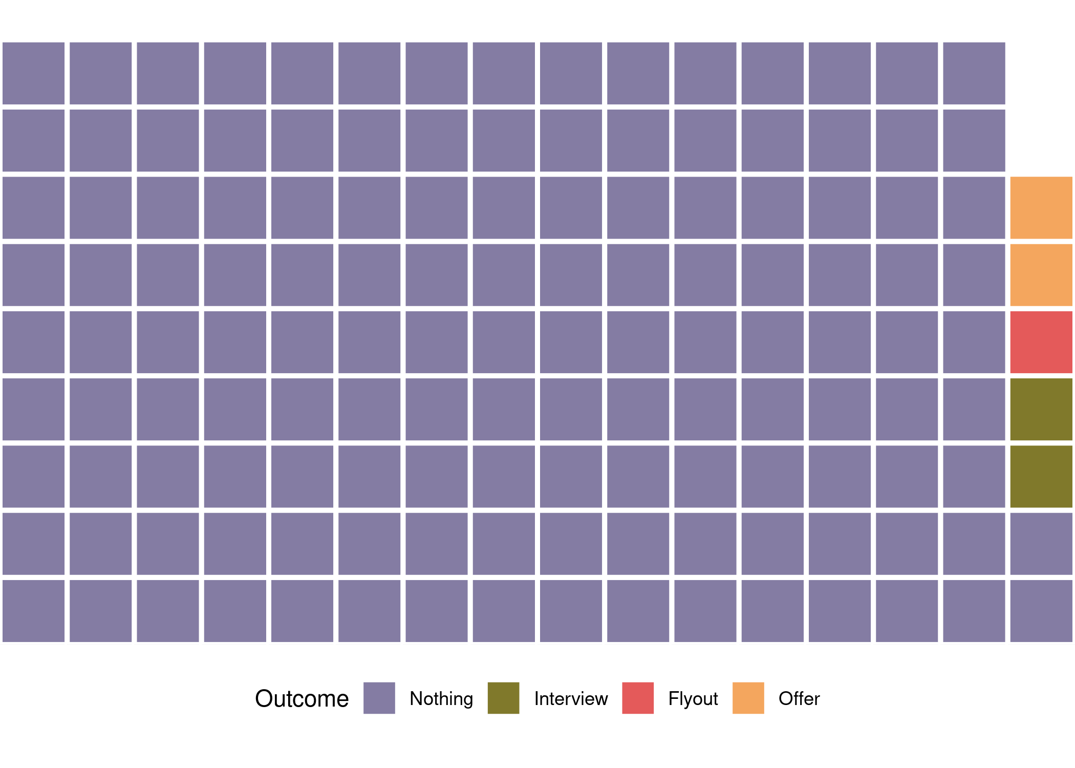
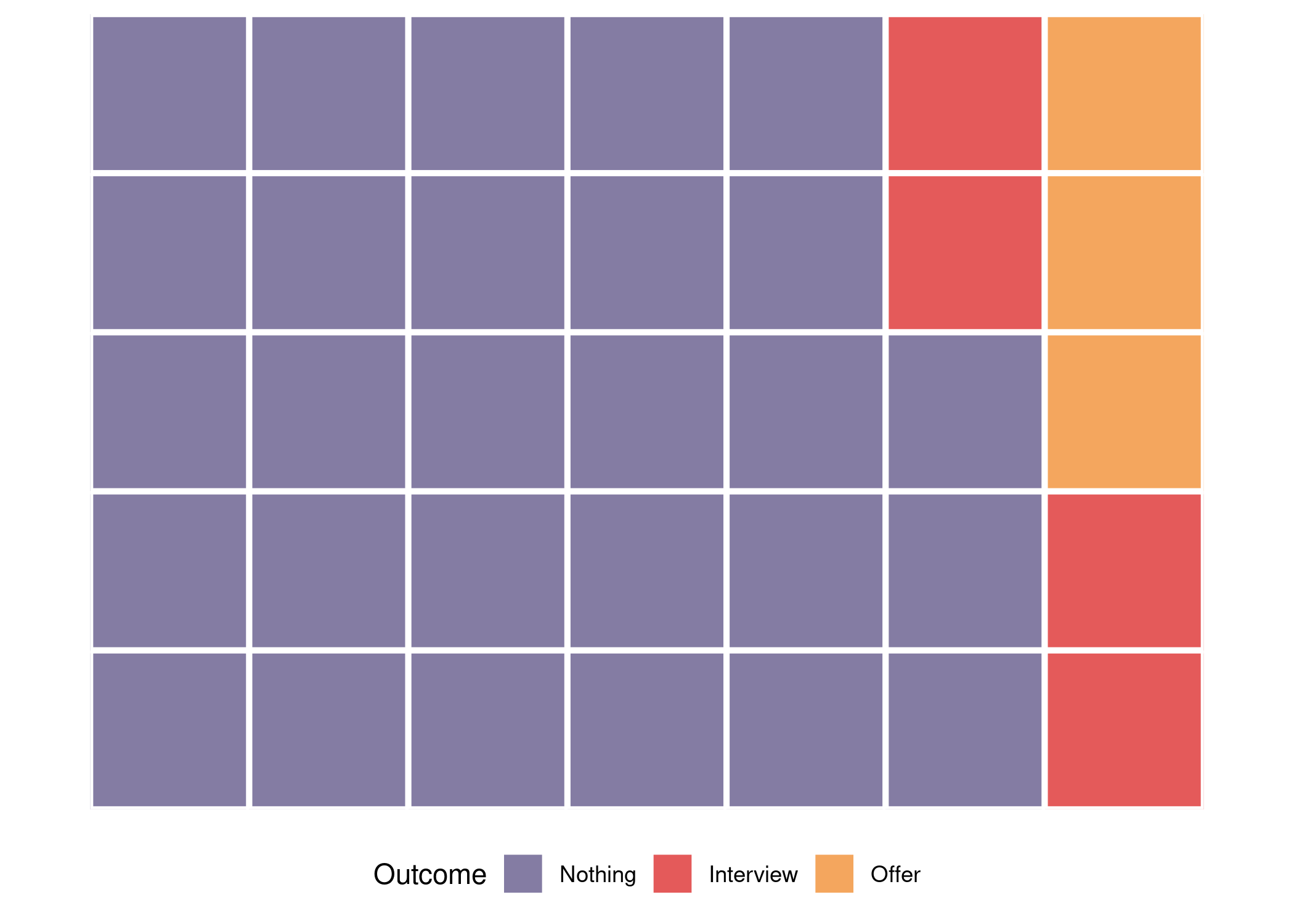
<p>Let’s get straight to the numbers. Out of 142 jobs I applied to, I
received two job offers. That’s a 98.6% rejection rate.<sup id="fnref:3" role="doc-noteref"><a href="#fn:3" class="footnote" rel="footnote">3</a></sup> Visualizing
this (with apologies to <a href="https://www.andrewheiss.com/blog/2018/12/17/academic-job-market-visualized">Andrew
Heiss</a>)
looks like so.</p>

<p><img src="/images/posts/so-it-goes/waffle_combined-1.png" style="display: block; margin: auto;" /></p>

<p>Five jobs expressed interest me beyond my initial application, which
translates to a 3.5% response rate. The ‘Nothing’ category encompasses
both jobs that sent me an automated HR rejection email (often several
months after their chosen candidate had accepted the offer) as well as
ones that never got back to me. Many searches for faculty positions will
conduct Zoom/Skype/Teams interviews with their long short list of
candidates before inviting the short list to an on-campus visit,
colloquially termed a flyout, but some may skip straight to the
on-campus visit. Some postdoc positions conduct virtual interviews,
while others simply make an offer to their preferred candidate. I used a
rough ranking of potential outcomes as Offer &gt; Flyout ≥ Interview
&gt; Rejection in constructing this plot, with each dot representing the
final outcome for that application.</p>

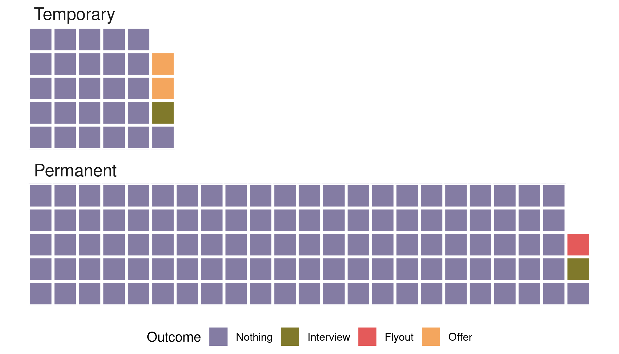
<p>I applied to a wide range of permanent (tenure-track and teaching-track)
faculty positions, as well as a number of temporary (postdoc, visiting
assistant professor, lecturer) positions. Splitting my applications
along this dimension shows that I had noticeably more success in my
applications for temporary positions (10.3% response rate) than
permanent ones (1.8% response rate).</p>

<p><img src="/images/posts/so-it-goes/waffle_split-1.png" style="display: block; margin: auto;" /></p>

<p>Since my non-nothing outcomes are so few, I can easily list them in more
detail:</p>

<ul>
  <li>Two postdoc offers</li>
  <li>A postdoc I interviewed for and declined in favor of another postdoc
offer</li>
  <li>A teaching-track flyout I declined in favor of a data science offer</li>
  <li>A tenure-track interview I declined in favor of the same offer</li>
</ul>

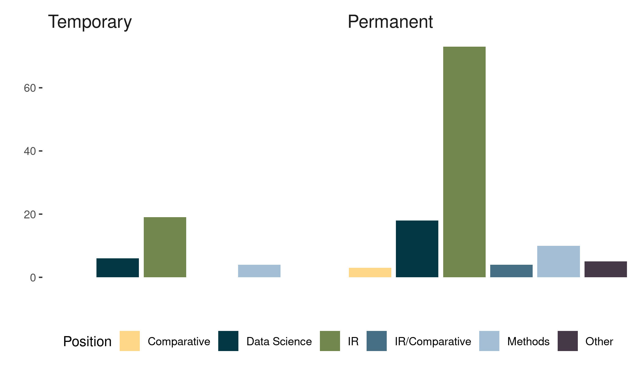
<p>If we break down the jobs I applied for by academic subfield, some
unsurprising patterns emerge. Data science jobs include those listed as
computational social science, jobs listed for a substantive subfield and
methods are coded under the substantive area, and international
relations, conflict, peace studies, security studies, and international
political economy are all represented in the IR category.</p>

<p><img src="/images/posts/so-it-goes/bar_subfield-1.png" style="display: block; margin: auto;" /></p>

<p>The majority of jobs I applied to (92) were advertised as international
relations. While much of my <a href="/research">research</a> sits at the
intersection of international relations and comparative politics, very
few of the jobs I applied to do. I didn’t track how frequent these jobs
are, so it could just be a case of few jobs to apply to. Data science
(24) handily outnumbers the more traditional subfield of methods (14),
reflecting increasing interest in the former by the discipline.</p>

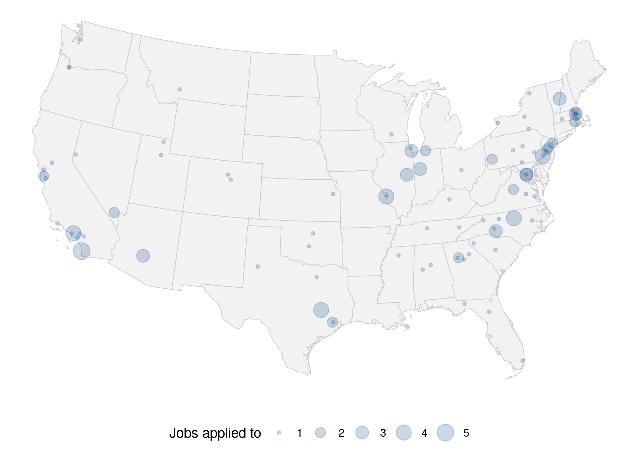
<p>The map below geographically visualizes the jobs I applied to. Each
circle represents one institution, with the size of the circle denoting
how many positions I applied for. I applied to five positions at UCSD,
the most of any institution.</p>

<p><img src="/images/posts/so-it-goes/map-1.png" style="display: block; margin: auto;" /></p>

<p>I focused primarily on the Eastern US and California. I applied to jobs
in 31 states and the District of Columbia, meaning there were 19 states
I did not apply to any jobs in. Looking at my applications over time
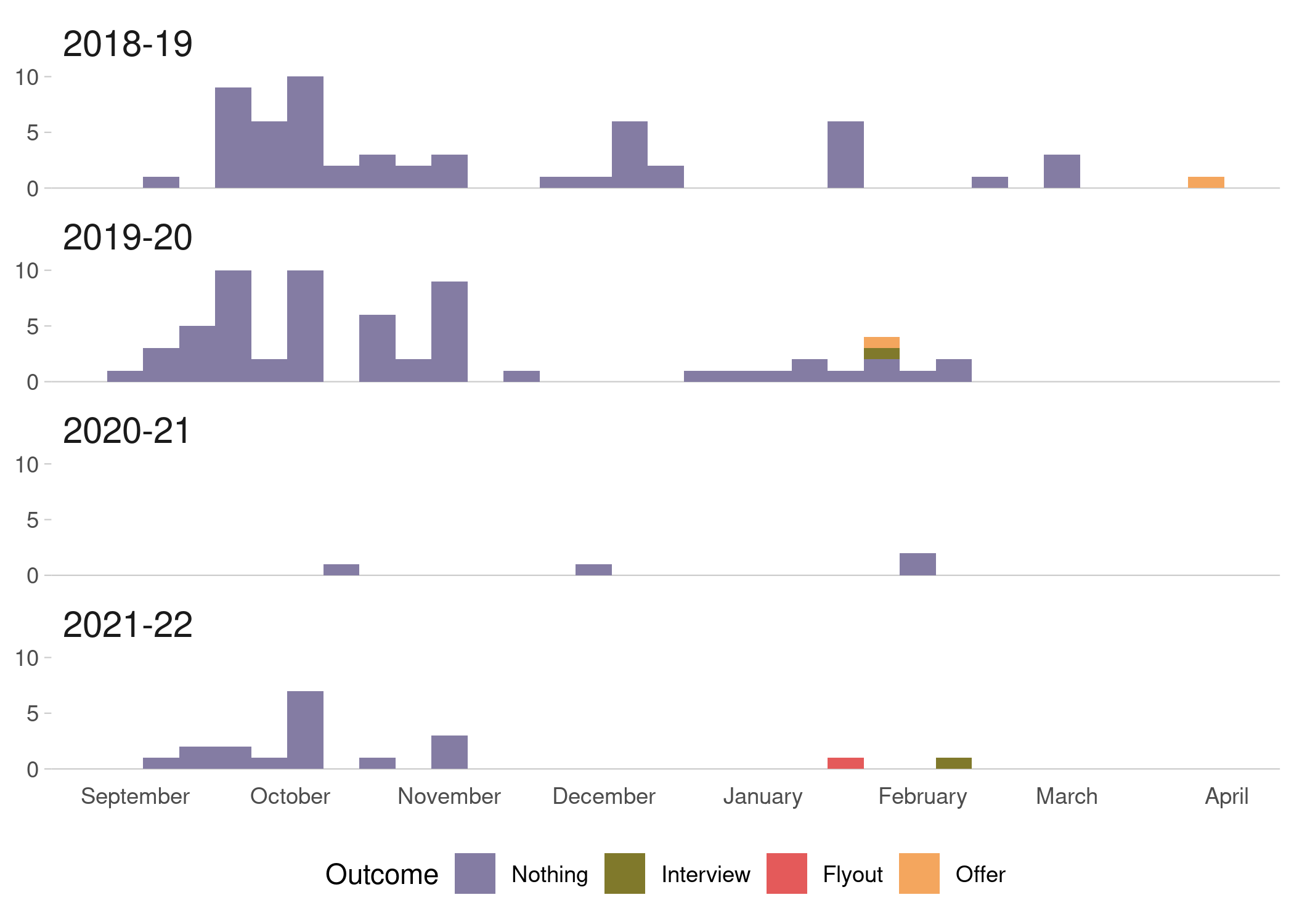
helps tell the story of my academic job search process.</p>

<p><img src="/images/posts/so-it-goes/date_hist-1.png" style="display: block; margin: auto;" /></p>

<p>The 2018-19 academic job market season was my final year of grad school.
I wanted to be done, so I applied to a wide variety of jobs. The postdoc
I received an offer from was actually the last position I applied for in
this cycle. I was a little more selective in the 2019-20 job market
season because I had an excellent postdoc, with a high chance of a
second year of funding. I started a new postdoc in 2020 and knew that I
had a second year of funding guaranteed. COVID-19 absolutely devastated
the job market that cycle as well. With a second year of funding secure
and precious few institutions hiring, I decided to spend my time
focusing on improving my CV and applied to a total of four jobs that
cycle, all tenure-track. The market somewhat recovered in the 2021-22
cycle, but there were still far fewer jobs than in my first two cycles.
I applied to 19 jobs this cycle, all of them permanent. There were some
great postdocs this cycle, but three years as a postdoc had been enough
for me.</p>

<p>Two jobs did show interest in me this last cycle, but it was too little,
too late. I had an offer for a data science job when I received an
on-campus interview for one job, and had already accepted the offer when
I received a Zoom interview for another. Given the typical pace of an
academic search, it was possible that even if I were successful in
getting an offer for either of these positions, it wouldn’t be for
another month or two. My postdoc ended in June, and an offer in hand
doing interesting research was an easy sell compared to that
uncertainty.</p>

<p>Across all 142 applications, I ended up submitting 399 letters of
recommendation to search committees. I was very fortunate that UNC has a
department administrator handle letters for grad students as a sort of
discount (read: free) Interfolio Dossier service. They generously
provide this service to graduates of the department until they secure
their first permanent job, even after they have left. I spent so long on
the academic job market that I had no less than three different people
help me with this process. I am incredibly grateful for their efforts
and want to highlight the support they gave me.</p>

<p>I haven’t done as good of a job tracking my applications to nonacademic
jobs because the process is much less structured and standardized. Some
applications require a cover letter, so I can count up all the cover
letters saved in my job search folder: 25. You can also apply for many
jobs with just a résumé. Let’s say I applied to 10 of those, which makes
35 applications total.</p>

<p><img src="/images/posts/so-it-goes/waffle_nonac-1.png" style="display: block; margin: auto;" /></p>

<p>I started the interview process with seven of these employers.
Acknowledging some uncertainty in the denominator, that’s a 20% response
rate, more than six times higher than my academic response rate of 3.5%.
I completed the interview process with four of these employers,
receiving one rejection and three offers (I withdrew from the other
three interview processes after accepting one of those offers). A 75%
interview success rate is pretty incredible compared to my experience on
the academic job market. That’s an overall success rate of 8.6%, which
is also more than six times higher than my overall success rate for
academic jobs.</p>

<p>Or is it a 50% success rate? I actually interviewed for two different
positions with two of these employers, so you could also slice the data
less favorably and say I received offers for three out of six positions
I interviewed for. That’s still an overall success rate of 8.1%, which
is pretty damn good in my eyes. I also want to highlight some of the
experiences I had on the nonacademic job market that I can’t imagine
ever happening on the academic one:</p>

<ul>
  <li>Recruiters reached out to me to ask me to apply to positions</li>
  <li>One employer alerted me to another position they were hiring for and
connected me with the hiring manager for it</li>
  <li>Another informed me that I was actually overqualified for the
position I applied for and considered me for a more senior position
instead</li>
  <li>I had my first job offer almost exactly three months after I started
my nonacademic job search in earnest</li>
  <li>I received three job offers in three days that week</li>
</ul>

<p>Others have written extensively about why you shouldn’t view a
nonacademic job as a backup option or a failure, but sometimes it’s just
nice to know that people want to pay you. If you’re striking out on the
academic job market, there are plenty of other options out there. So it
goes.</p>

<div class="footnotes" role="doc-endnotes">
  <ol>
    <li id="fn:1" role="doc-endnote">
      <p>People have criticized the term quit lit for focusing on the
individual and <a href="https://www.wihe.com/article-details/74/quit-lit-is-about-labor-conditions">ignoring the systemic
forces</a>
that contribute to many people’s decision to leave academia. I am
very persuaded by this argument, but no one has yet coined a
similarly catchy and succinct alternative. <a href="#fnref:1" class="reversefootnote" role="doc-backlink">&#8617;</a></p>
    </li>
    <li id="fn:2" role="doc-endnote">
      <p>I’m using the term nonacademic instead of industry, which is
usually presented as the alternative to academic jobs for people
with a PhD, because I applied for jobs in both the private and
public sectors. <a href="#fnref:2" class="reversefootnote" role="doc-backlink">&#8617;</a></p>
    </li>
    <li id="fn:3" role="doc-endnote">
      <p>I considered Kilgore Trout’s intended epitaph from <em>Breakfast of
Champions</em> as a title for this post, but decided it was both too
obscure and too bleak: he tried. <a href="#fnref:3" class="reversefootnote" role="doc-backlink">&#8617;</a></p>
    </li>
  </ol>
</div>]]></content><author><name>Dany Laksono</name><email>dany.laksono@city.ac.uk</email></author><category term="career" /><category term="data-science" /><category term="visualization" /><summary type="html"><![CDATA[When I was applying to graduate school and asking for letters of recommendation from my undergrad professors, one of them told me to give academia three years, and that if I hadn’t found a permanent position by then, to find another career. It’s been three years, and next week I start a new job as a data scientist. I read a fair bit of quit lit in my first couple years of grad school and always told myself that if I went that same route, I would never pen any of my own…]]></summary></entry><entry><title type="html">Regular expressions for replication</title><link href="https://danylaksono.is-a.dev/posts/2021/07-rstudio-regex" rel="alternate" type="text/html" title="Regular expressions for replication" /><published>2021-07-01T00:00:00-05:00</published><updated>2021-07-01T00:00:00-05:00</updated><id>https://danylaksono.is-a.dev/posts/2021/rstudio-regex</id><content type="html" xml:base="https://danylaksono.is-a.dev/posts/2021/07-rstudio-regex"><![CDATA[<p>As part of the publication process for my recent <a href="https://doi.org/10.1177/07388942211015242">article</a> on how states preempt separatist conflict, I needed to submit replication materials to the journal. I took my graduate quantitative methods sequence with the late <a href="https://sites.google.com/view/tom-carsey/home">Tom Carsey</a>, so I’ve long been a proponent replicability efforts in social science. I also had an hourly job in grad school replicating quantitative results for multiple political science journals, so I’m very familiar with best practices for replication. Unfortunately, in the four years since I wrote the first line of code for this project, somewhere in between defending my dissertation and starting a new job (ok, fine, almost immediately after writing that first line of code), I got a little lazy.</p>

<!--more-->

<p>Sometimes it’s faster (easier) to just write code that works for you, on your system, without any consideration for some poor researcher who may try to replicate your results in the future.<sup id="fnref:replication" role="doc-noteref"><a href="#fn:replication" class="footnote" rel="footnote">1</a></sup> This tendency was especially bad for this project because at various points in time I was writing code to run on my personal laptop and <a href="https://its.unc.edu/research-computing/killdevil-retirement/">two</a> <a href="https://its.unc.edu/research-computing/longleaf-cluster/">different</a> high performance computing clusters. This is a recipe for code that doesn’t travel well and will almost certainly fail to replicate.</p>

<p>There were a lot of changes I made to my code to ensure my results replicate, but the most tedious (and time consuming, by far) was cleaning up my file paths. Due to the computationally intensive GIS work and Bayesian statistics involved in the project, I ran lots of code on a cluster, and then pulled the results back to my laptop to summarize and create figures. This unsurprisingly resulted in a huge mess when looking at the project as a whole, rather than any individual script. Luckily, R and Rstudio made things (relatively) painless to fix.</p>

<h1 id="file-paths">File paths</h1>

<p>Anytime you load a dataset into R, you need to specify the path to that file. The same’s true when you save R output to a file. This article started as a chapter of my dissertation, so all of the code originally lived in the Dissertation folder on my laptop. However, as I started adapting it to an article length manuscript, I created a new Conflict Preemption folder in my Projects folder. By the time the article was accepted, I had two main folders I needed to combine:</p>

<ul>
  <li><code class="language-plaintext highlighter-rouge">/Users/Rob/Dropbox/UNC/Dissertation/Onset</code></li>
  <li><code class="language-plaintext highlighter-rouge">/Users/Rob/Dropbox/WashU/Projects/Conflict Preemption</code></li>
</ul>

<p>Both of these folders live in my Dropbox, but that’s about where the similarities end. I wrote most of the code for running models while still at UNC, so when I added new scripts to run models to respond to reviewer comments, I still stuck them in the UNC folder. That also means that all of the output of these models ended up in the UNC folder when it got transferred from the cluster. However, when I needed to do something simpler like create a time series plot of the number of separatist groups in existence, I wrote that code in the WashU folder. I also had a script in the WashU folder to load all of the results and generate plots from them. Because this script and the data it needed to load where in completely different directories, this is what I had to do to load the data to create one of the main figures:</p>

<div class="language-r highlighter-rouge"><div class="highlight"><pre class="highlight"><code><span class="n">load</span><span class="p">(</span><span class="s1">'/Users/Rob/Dropbox/UNC/Dissertation/Onset/Figure Data/marg_eff_pop_df_cy.RData'</span><span class="p">)</span><span class="w">
</span></code></pre></div></div>

<p>Not particularly likely to work on anyone else’s computer. To fix this, I needed to move all of the data to the Conflict Preemption folder, which was easy, and then rewrite all of the code the referenced file locations, which was less easy.</p>

<h1 id="here">Here</h1>

<p>As a first step, I needed to chop off <code class="language-plaintext highlighter-rouge">/Users/Rob/Dropbox/UNC/Dissertation/Onset/</code> from the start of every file path. All the files for the article, including both the R scripts and the various data files, now live in <code class="language-plaintext highlighter-rouge">/Users/Rob/Dropbox/WashU/Projects/Conflict Preemption</code>, but all of the file paths in the scripts still start with <code class="language-plaintext highlighter-rouge">/Users/Rob/Dropbox/UNC/Dissertation/Onset</code>, because that’s where all the files were before. You can do this just using the standard find and replace functionality built into RStudio. However, there’s no guarantee that someone in the future will correctly set R’s working directory before running the code. I used the <a href="https://here.r-lib.org/">here</a> R package to ensure that R can always find everything it needs for my code. All you have to do is wrap file paths in the <code class="language-plaintext highlighter-rouge">here()</code> function in the package, and they’ll be automatically completed with the full file path, letting R find your files.<sup id="fnref:here" role="doc-noteref"><a href="#fn:here" class="footnote" rel="footnote">2</a></sup></p>

<p>You need to use the <a href="https://en.wikipedia.org/wiki/Path_(computing)#Absolute_and_relative_paths">relative path</a> to each file, so for a file with an absolute path of <code class="language-plaintext highlighter-rouge">/Users/Rob/Dropbox/WashU/Projects/Conflict Preemption/Figure Data/marg_eff_pop_df_cy.RData</code>, the relative path (relative to the project folder of <code class="language-plaintext highlighter-rouge">/Users/Rob/Dropbox/WashU/Projects/Conflict Preemption</code>) would be <code class="language-plaintext highlighter-rouge">Figure Data/marg_eff_pop_df_cy.RData</code>. The final bit of R code looks like this:</p>

<div class="language-r highlighter-rouge"><div class="highlight"><pre class="highlight"><code><span class="n">load</span><span class="p">(</span><span class="n">here</span><span class="p">(</span><span class="s1">'Figure Data/marg_eff_pop_df_cy.RData'</span><span class="p">))</span><span class="w">
</span></code></pre></div></div>

<p>The addition of that <code class="language-plaintext highlighter-rouge">here()</code> in between <code class="language-plaintext highlighter-rouge">load()</code> and the file path means that things are no longer as simple as finding and replacing the start of the file path.</p>

<h1 id="regular-expressions">Regular expressions</h1>

<p>Luckily, I was able to take advantage of RStudio’s built in support for <a href="https://en.wikipedia.org/wiki/Regular_expression">regular expressions</a> to save myself from having to manually change each line of code that either loaded or saved a file. Regular expressions are a powerful way to search through and manipulate text. You can activate them in RStudio’s find and replace dialog by checking the Regex box:</p>

<p><img src="/images/posts/rstudio-regex/regex.png" alt="" class="align-center" /></p>

<p>Once you’ve done that, certain characters in your search will no longer be interpreted literally. The most important difference is probably <code class="language-plaintext highlighter-rouge">.</code>, which is a stand-in for any character.<sup id="fnref:newline" role="doc-noteref"><a href="#fn:newline" class="footnote" rel="footnote">3</a></sup> This is similar to how <code class="language-plaintext highlighter-rouge">*</code> is a wildcard in the Unix shell, e.g., you can use <code class="language-plaintext highlighter-rouge">ls *.R</code> to list all R script files in a folder. The main regular expression feature I used is the <a href="https://www.regular-expressions.info/refcapture.html">capturing group</a>, which allows you to identify and extract a subset of a line of text. You designate a capturing group by surrounding the desired text with parentheses. To fix all of the code loading RData files from the Figure Data folder, my regular expression looked like this:</p>

<div class="language-plaintext highlighter-rouge"><div class="highlight"><pre class="highlight"><code>'/Users/Rob/Dropbox/UNC/Dissertation/Onset/(Figure Data/.*\.RData)'
</code></pre></div></div>

<p>It starts with <code class="language-plaintext highlighter-rouge">/Users/Rob/Dropbox/UNC/Dissertation/Onset/</code>, which is the part I want to get rid of. Next, <code class="language-plaintext highlighter-rouge">(Figure Data/.*\.RData)'</code> tells the regular expression to look for any character (<code class="language-plaintext highlighter-rouge">.</code>) repeated an unlimited number of times (<code class="language-plaintext highlighter-rouge">*</code>) followed by <code class="language-plaintext highlighter-rouge">.RData</code>. Because <code class="language-plaintext highlighter-rouge">.</code> is a special character in regular expressions, we have to escape it with a backslash (<code class="language-plaintext highlighter-rouge">\</code>). This will match any file name ending in <code class="language-plaintext highlighter-rouge">.RData</code> in the Figure Data folder. If we left out the leading <code class="language-plaintext highlighter-rouge">/Users/Rob/Dropbox/UNC/Dissertation/Onset/</code>, we end up with the capturing group we want, but since <code class="language-plaintext highlighter-rouge">/Users/Rob/Dropbox/UNC/Dissertation/Onset/</code> wouldn’t be part of the search string, it wouldn’t end up getting replaced. This is the same reason we need to include the opening and closing quotation marks; if we didn’t, we’d end up with a <code class="language-plaintext highlighter-rouge">here()</code> command inside quotation marks, which R would just treat as a string and not a command.</p>

<p>At this point I had the core of the line that I wanted to keep, but now I needed to extract it and place it inside of a call to <code class="language-plaintext highlighter-rouge">here()</code>. You accomplish this goal using a <a href="https://www.regular-expressions.info/replacebackref.html">backreference</a> to the capturing group. To reference the first capturing group, you use either <code class="language-plaintext highlighter-rouge">\1</code> or <code class="language-plaintext highlighter-rouge">$1</code> depending on which version of regular expressions you are using. This is often very difficult to figure out, and is one of the most annoying things about regular expressions. You’ll often just have to experiment and find out which one to use through trial and error. Luckily RStudio accepts either version!</p>

<p>To replace the absolute path with a relative one wrapped in a <code class="language-plaintext highlighter-rouge">here()</code> call, this is what I typed into the Replace field in the find and replace dialog:</p>

<div class="language-plaintext highlighter-rouge"><div class="highlight"><pre class="highlight"><code>here('$1')
</code></pre></div></div>

<p>and it resulted in this:</p>

<div class="language-r highlighter-rouge"><div class="highlight"><pre class="highlight"><code><span class="n">here</span><span class="p">(</span><span class="s1">'Figure Data/marg_eff_pop_df_cy.RData'</span><span class="p">)</span><span class="w">
</span></code></pre></div></div>

<p>Thanks to the power of capture groups, you can just hit the replace all button and instantly transform every file path into a much more portable and replication-friendly one.</p>

<h1 id="a-little-bit-faster-now">A little bit faster now</h1>

<p>If you’re feeling really confident that you moved every file correctly, you can replace <em>all</em> file paths with the following regular expression:</p>

<div class="language-plaintext highlighter-rouge"><div class="highlight"><pre class="highlight"><code>'/Users/Rob/Dropbox/UNC/Dissertation/Onset/(.*\..*)'
</code></pre></div></div>

<p>This will get any files with file extensions (the <code class="language-plaintext highlighter-rouge">\.</code> followed by <code class="language-plaintext highlighter-rouge">.*</code> to ensure there’s at least one character after a literal period), as well as any preceding subdirectories (the initial <code class="language-plaintext highlighter-rouge">.*</code>) and stick them all into the resulting <code class="language-plaintext highlighter-rouge">here()</code> call. As an example, this will successfully turn this:
fileConn &lt;- file(here::here(‘Tables/pd_pop_cy.tex’))</p>

<div class="language-r highlighter-rouge"><div class="highlight"><pre class="highlight"><code><span class="n">groups</span><span class="w"> </span><span class="o">&lt;-</span><span class="w"> </span><span class="n">readRDS</span><span class="p">(</span><span class="s1">'/Users/Rob/Dropbox/Dissertation/Onset/Input Data/groups_nightlights.RDS'</span><span class="p">)</span><span class="w">
</span></code></pre></div></div>

<p>into this:</p>

<div class="language-r highlighter-rouge"><div class="highlight"><pre class="highlight"><code><span class="n">groups</span><span class="w"> </span><span class="o">&lt;-</span><span class="w"> </span><span class="n">readRDS</span><span class="p">(</span><span class="n">here</span><span class="o">::</span><span class="n">here</span><span class="p">(</span><span class="s1">'Input Data/groups_nightlights.RDS'</span><span class="p">))</span><span class="w">
</span></code></pre></div></div>
<div class="footnotes" role="doc-endnotes">
  <ol>
    <li id="fn:replication" role="doc-endnote">
      <p>I’m using ‘replication’ here to mean that the code used to generate quantitative results from a dataset should produce those same results when run by another researcher, <em>not</em> in the sense that means that independent researchers following the published protocol can collect the data themselves and arrive at the same conclusion. I use the term ‘reproducible’ to describe this property. Annoyingly, different fields use <a href="https://www.ncbi.nlm.nih.gov/books/NBK547546/">opposing definitions</a> of these two terms. <a href="#fnref:replication" class="reversefootnote" role="doc-backlink">&#8617;</a></p>
    </li>
    <li id="fn:here" role="doc-endnote">
      <p>Specifically, <code class="language-plaintext highlighter-rouge">here()</code> will key into the <code class="language-plaintext highlighter-rouge">.Rproj</code> file included in my replication materials and use that to properly locate everything else. <a href="#fnref:here" class="reversefootnote" role="doc-backlink">&#8617;</a></p>
    </li>
    <li id="fn:newline" role="doc-endnote">
      <p>Except for newlines, carriage returns, and other end of line special characters. <a href="#fnref:newline" class="reversefootnote" role="doc-backlink">&#8617;</a></p>
    </li>
  </ol>
</div>]]></content><author><name>Dany Laksono</name><email>dany.laksono@city.ac.uk</email></author><category term="regex" /><summary type="html"><![CDATA[As part of the publication process for my recent article on how states preempt separatist conflict, I needed to submit replication materials to the journal. I took my graduate quantitative methods sequence with the late Tom Carsey, so I’ve long been a proponent replicability efforts in social science. I also had an hourly job in grad school replicating quantitative results for multiple political science journals, so I’m very familiar with best practices for replication. Unfortunately, in the four years since I wrote the first line of code for this project, somewhere in between defending my dissertation and starting a new job (ok, fine, almost immediately after writing that first line of code), I got a little lazy.]]></summary></entry><entry><title type="html">Faceted maps in R</title><link href="https://danylaksono.is-a.dev/posts/2021/05/geom-sf-facet" rel="alternate" type="text/html" title="Faceted maps in R" /><published>2021-05-19T00:00:00-05:00</published><updated>2021-05-19T00:00:00-05:00</updated><id>https://danylaksono.is-a.dev/posts/2021/05/geom-sf-facet</id><content type="html" xml:base="https://danylaksono.is-a.dev/posts/2021/05/geom-sf-facet"><![CDATA[<p>I recently needed to create a choropleth of a few different countries
for a project on targeting of UN peacekeepers by non-state armed actors
I’m working on. A
<a href="https://en.wikipedia.org/wiki/Choropleth_map">choropleth</a> is a type of
thematic map where data are aggregated up from smaller areas (or
discrete points) to larger ones and then visualized using different
colors to represent different numeric values.</p>

<!--more-->

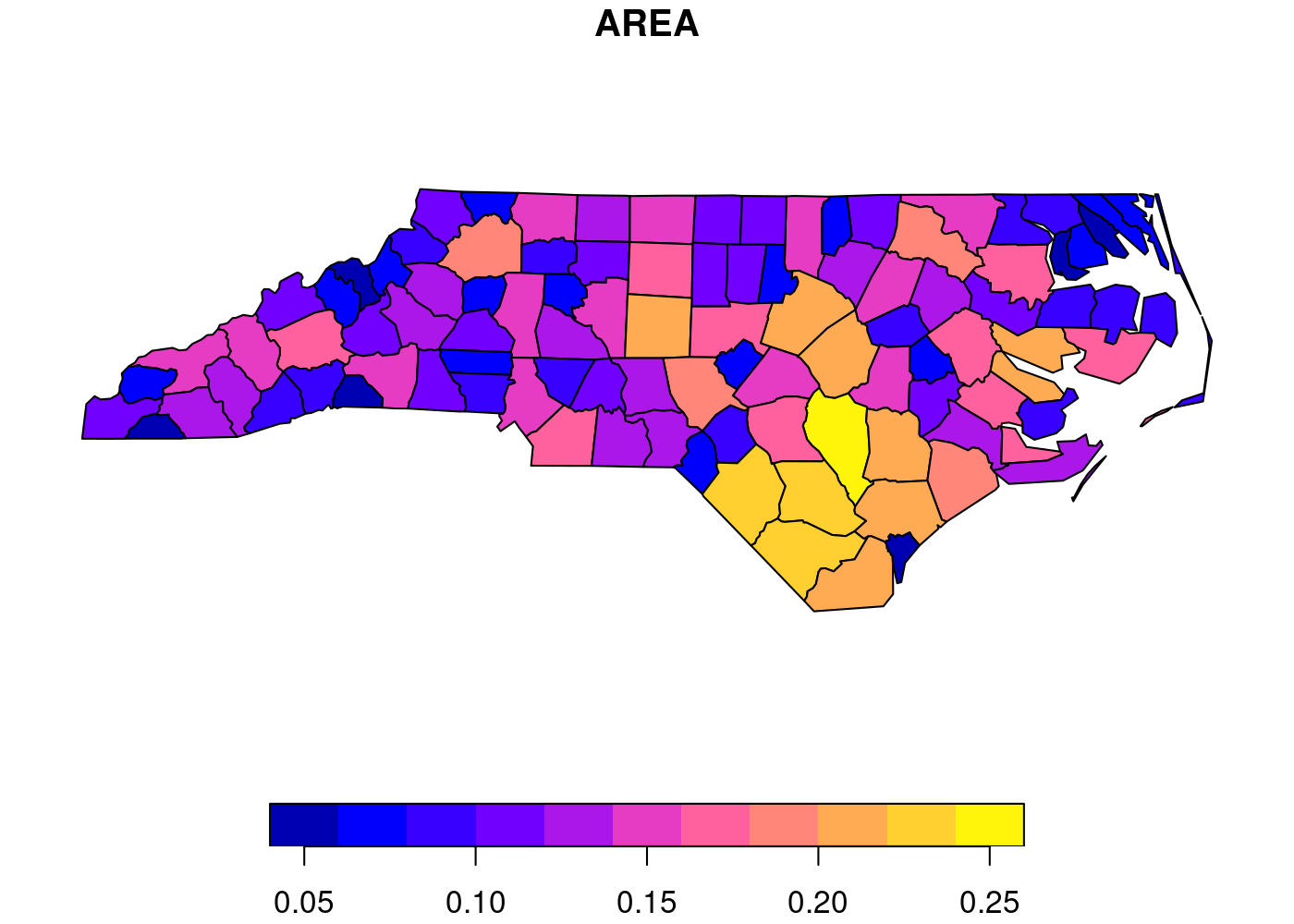
<p>See this simple example, which displays the area of each county in North
Carolina, from the <code class="language-plaintext highlighter-rouge">sf</code> package
<a href="https://r-spatial.github.io/sf/articles/sf1.html#sfc-simple-feature-geometry-list-column-1">documentation</a>.<sup id="fnref:1" role="doc-noteref"><a href="#fn:1" class="footnote" rel="footnote">1</a></sup>
First, we need to load <code class="language-plaintext highlighter-rouge">sf</code> and then get the built-in <code class="language-plaintext highlighter-rouge">nc</code> dataset:</p>

<div class="language-r highlighter-rouge"><div class="highlight"><pre class="highlight"><code><span class="n">library</span><span class="p">(</span><span class="n">sf</span><span class="p">)</span><span class="w">
</span><span class="n">nc</span><span class="w"> </span><span class="o">&lt;-</span><span class="w"> </span><span class="n">st_read</span><span class="p">(</span><span class="n">system.file</span><span class="p">(</span><span class="s1">'shape/nc.shp'</span><span class="p">,</span><span class="w"> </span><span class="n">package</span><span class="w"> </span><span class="o">=</span><span class="w"> </span><span class="s1">'sf'</span><span class="p">))</span><span class="w">
</span><span class="n">plot</span><span class="p">(</span><span class="n">nc</span><span class="p">[</span><span class="m">1</span><span class="p">])</span><span class="w">
</span></code></pre></div></div>

<p><img src="/images/posts/geom-sf-facet/nc-1.png" style="display: block; margin: auto;" />
Since I needed to generate choropleths for multiple countries, I decided
to use <code class="language-plaintext highlighter-rouge">ggplot2</code>’s powerful
<a href="https://ggplot2.tidyverse.org/reference/facet_grid.html">faceting</a>
functionality. Unfortunately, as I discuss
<a href="#first-attempt-ggplot2">below</a>, <code class="language-plaintext highlighter-rouge">ggplot2</code> and <code class="language-plaintext highlighter-rouge">sf</code> don’t work together
perfectly in ways that become more apparent (and problematic) the more
complex your plots get. I moved away from faceting, and just glued
together a bunch of separate plots, but then I had to figure out how to
end up with a shared legend for five separate plots. Read on to see how
I solved both of these issues.</p>

<h1 id="the-data">The data</h1>

<p>I already loaded <code class="language-plaintext highlighter-rouge">sf</code> to make the plot of North Carolina above, so now
let’s load the remaining packages we’ll use:</p>

<div class="language-r highlighter-rouge"><div class="highlight"><pre class="highlight"><code><span class="n">library</span><span class="p">(</span><span class="n">tidyverse</span><span class="p">)</span><span class="w"> </span><span class="c1"># data manipulation and plotting</span><span class="w">
</span><span class="n">library</span><span class="p">(</span><span class="n">tmap</span><span class="p">)</span><span class="w">      </span><span class="c1"># spatial plots</span><span class="w">
</span><span class="n">library</span><span class="p">(</span><span class="n">cowplot</span><span class="p">)</span><span class="w">   </span><span class="c1"># combine plots</span><span class="w">
</span><span class="n">library</span><span class="p">(</span><span class="n">RWmisc</span><span class="p">)</span><span class="w">    </span><span class="c1"># clean plot theme</span><span class="w">
</span></code></pre></div></div>

<p>I’m working with cleaned and subsetted versions of
<a href="https://acleddata.com/">ACLED</a> and <a href="https://gadm.org/">GADM</a>, which
I’ve uploaded to my website as <code class="language-plaintext highlighter-rouge">PKO.Rdata</code> if you want to download them
and run this code yourself. The <code class="language-plaintext highlighter-rouge">acled</code> object contains a list of
attacks on peacekeepers in active Chapter VII UN peacekeeping missions
in Subsaharan Africa, while the <code class="language-plaintext highlighter-rouge">adm</code> object contains all of the second
order administrative districts (ADM2) in the five countries with active
missions.</p>

<div class="language-r highlighter-rouge"><div class="highlight"><pre class="highlight"><code><span class="c1">## load data</span><span class="w">
</span><span class="n">load</span><span class="p">(</span><span class="n">url</span><span class="p">(</span><span class="s1">'https://jayrobwilliams.com/data/PKO.Rdata'</span><span class="p">))</span><span class="w">

</span><span class="c1">## inspect</span><span class="w">
</span><span class="n">head</span><span class="p">(</span><span class="n">acled</span><span class="p">)</span><span class="w">
</span><span class="n">head</span><span class="p">(</span><span class="n">adm</span><span class="p">)</span><span class="w">
</span></code></pre></div></div>

<div class="language-plaintext highlighter-rouge"><div class="highlight"><pre class="highlight"><code>## Simple feature collection with 6 features and 30 fields
## Geometry type: POINT
## Dimension:     XY
## Bounding box:  xmin: -3.6102 ymin: 0.4966 xmax: 29.4654 ymax: 19.4695
## Geodetic CRS:  WGS 84
## # A tibble: 6 x 31
##   data_id   iso event_id_cnty event_id_no_cnty event_date  year time_precision
##     &lt;dbl&gt; &lt;dbl&gt; &lt;chr&gt;                    &lt;dbl&gt; &lt;date&gt;     &lt;dbl&gt;          &lt;dbl&gt;
## 1 6713346   140 CEN47283                 47283 2019-12-27  2019              1
## 2 6689432   180 DRC16211                 16211 2019-12-08  2019              1
## 3 7578005   180 DRC16182                 16182 2019-12-04  2019              1
## 4 7191069   466 MLI3253                   3253 2019-10-21  2019              1
## 5 6759702   466 MLI3225                   3225 2019-10-06  2019              1
## 6 6023339   466 MLI3224                   3224 2019-10-06  2019              1
## # … with 24 more variables: event_type &lt;chr&gt;, sub_event_type &lt;chr&gt;,
## #   actor1 &lt;chr&gt;, assoc_actor_1 &lt;chr&gt;, inter1 &lt;dbl&gt;, actor2 &lt;chr&gt;,
## #   assoc_actor_2 &lt;chr&gt;, inter2 &lt;dbl&gt;, interaction &lt;dbl&gt;, region &lt;chr&gt;,
## #   country &lt;chr&gt;, admin1 &lt;chr&gt;, admin2 &lt;chr&gt;, admin3 &lt;chr&gt;, location &lt;chr&gt;,
## #   geo_precision &lt;dbl&gt;, source &lt;chr&gt;, source_scale &lt;chr&gt;, notes &lt;chr&gt;,
## #   fatalities &lt;dbl&gt;, timestamp &lt;dbl&gt;, iso3 &lt;chr&gt;, month &lt;dbl&gt;,
## #   geometry &lt;POINT [°]&gt;

## Simple feature collection with 6 features and 19 fields
## Geometry type: MULTIPOLYGON
## Dimension:     XY
## Bounding box:  xmin: 18.54607 ymin: 4.221635 xmax: 22.395 ymax: 9.774724
## Geodetic CRS:  WGS 84
## # A tibble: 6 x 20
##   GID_0 NAME_0   GID_1  NAME_1 NL_NAME_1 GID_2 NAME_2 VARNAME_2 NL_NAME_2 TYPE_2
##   &lt;chr&gt; &lt;chr&gt;    &lt;chr&gt;  &lt;chr&gt;  &lt;chr&gt;     &lt;chr&gt; &lt;chr&gt;  &lt;chr&gt;     &lt;chr&gt;     &lt;chr&gt; 
## 1 CAF   Central… CAF.1… Bamin… &lt;NA&gt;      CAF.… Bamin… &lt;NA&gt;      &lt;NA&gt;      Sous-…
## 2 CAF   Central… CAF.1… Bamin… &lt;NA&gt;      CAF.… Ndélé  &lt;NA&gt;      &lt;NA&gt;      Sous-…
## 3 CAF   Central… CAF.2… Bangui &lt;NA&gt;      CAF.… Bangui &lt;NA&gt;      &lt;NA&gt;      Sous-…
## 4 CAF   Central… CAF.3… Basse… &lt;NA&gt;      CAF.… Alind… &lt;NA&gt;      &lt;NA&gt;      Sous-…
## 5 CAF   Central… CAF.3… Basse… &lt;NA&gt;      CAF.… Kembé  &lt;NA&gt;      &lt;NA&gt;      Sous-…
## 6 CAF   Central… CAF.3… Basse… &lt;NA&gt;      CAF.… Minga… &lt;NA&gt;      &lt;NA&gt;      Sous-…
## # … with 10 more variables: ENGTYPE_2 &lt;chr&gt;, CC_2 &lt;chr&gt;, HASC_2 &lt;chr&gt;,
## #   ID_0 &lt;dbl&gt;, ISO &lt;chr&gt;, ID_1 &lt;dbl&gt;, ID_2 &lt;dbl&gt;, CCN_2 &lt;dbl&gt;, CCA_2 &lt;chr&gt;,
## #   geometry &lt;MULTIPOLYGON [°]&gt;
</code></pre></div></div>

<h1 id="first-attempt-ggplot2">First attempt: <code class="language-plaintext highlighter-rouge">ggplot2</code></h1>

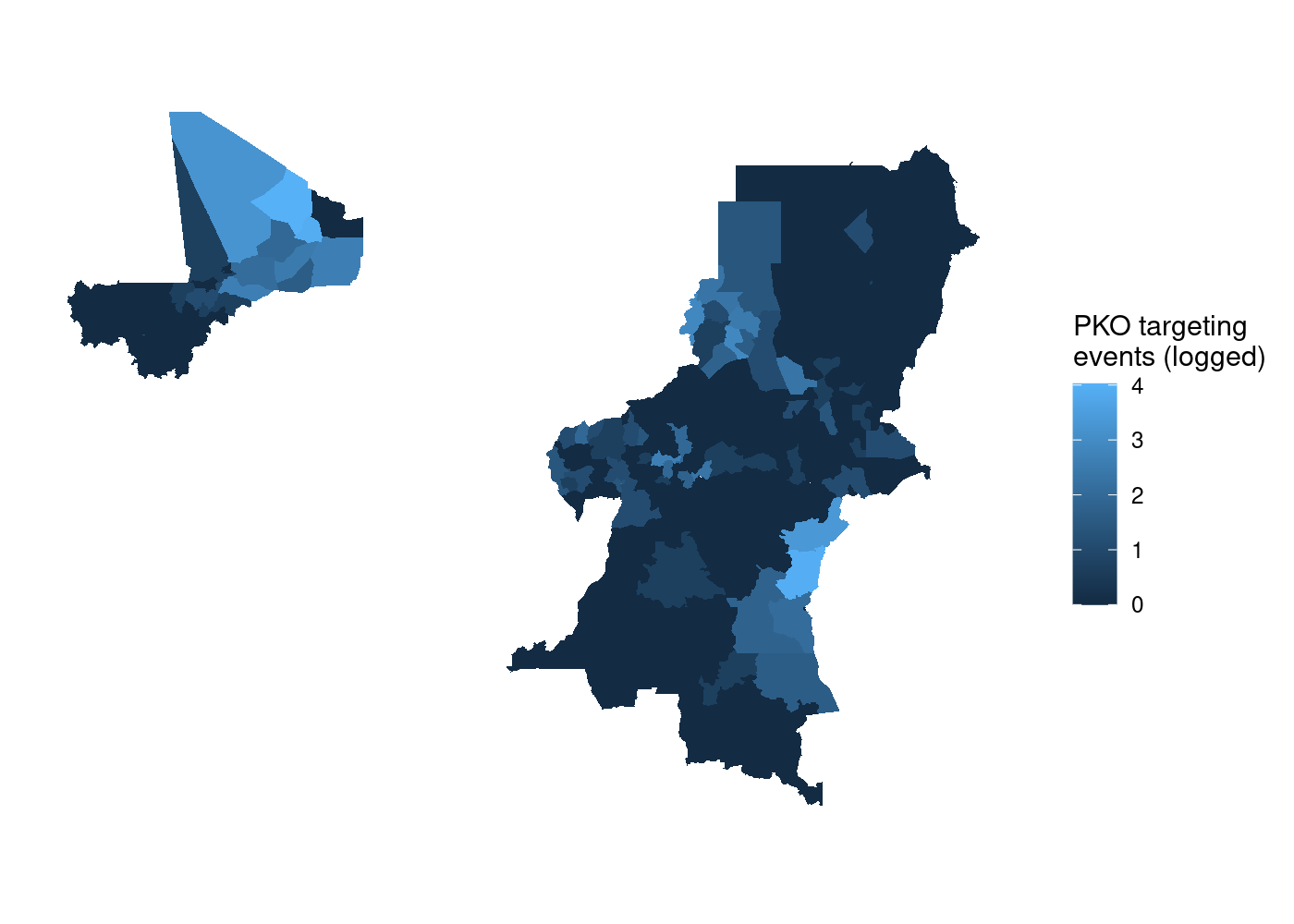
<p>The first step we need to do is associate each individual attack with
the ADM2 it occurred in. We can do this with the <code class="language-plaintext highlighter-rouge">st_join()</code> function.
This function executes a left join by default, so by using <code class="language-plaintext highlighter-rouge">adm</code> for the
<code class="language-plaintext highlighter-rouge">x</code> argument and <code class="language-plaintext highlighter-rouge">acled</code> for the <code class="language-plaintext highlighter-rouge">y</code> argument, we end up with one row
for every ADM2 with no attacks in it, and <em>n</em> rows for each ADM2 with
attacks in it, where <em>n</em> equals the number of attacks in that ADM2. We
can then use <code class="language-plaintext highlighter-rouge">group_by()</code> and <code class="language-plaintext highlighter-rouge">summarize()</code> to create a count of attacks
for each ADM2 by summing the number of non-NA observations of
<code class="language-plaintext highlighter-rouge">event_id_cnty</code>, the main ID field in ACLED. Finally, I log this count
variable (using <code class="language-plaintext highlighter-rouge">log1p()</code> to account for the ADM2s without any attacks
because <em>ln</em>(0) is undefined) to make the resulting plot more
informative due to outliers in Northern Mali and the Eastern DRC.
Putting it all together:</p>

<div class="language-r highlighter-rouge"><div class="highlight"><pre class="highlight"><code><span class="n">st_join</span><span class="p">(</span><span class="n">adm</span><span class="p">,</span><span class="w"> </span><span class="n">acled</span><span class="p">)</span><span class="w"> </span><span class="o">%&gt;%</span><span class="w"> 
  </span><span class="n">group_by</span><span class="p">(</span><span class="n">NAME_0</span><span class="p">,</span><span class="w"> </span><span class="n">NAME_1</span><span class="p">,</span><span class="w"> </span><span class="n">NAME_2</span><span class="p">)</span><span class="w"> </span><span class="o">%&gt;%</span><span class="w"> 
  </span><span class="n">summarize</span><span class="p">(</span><span class="n">attacks</span><span class="w"> </span><span class="o">=</span><span class="w"> </span><span class="n">log1p</span><span class="p">(</span><span class="nf">sum</span><span class="p">(</span><span class="o">!</span><span class="nf">is.na</span><span class="p">(</span><span class="n">event_id_cnty</span><span class="p">))))</span><span class="w"> </span><span class="o">%&gt;%</span><span class="w"> 
  </span><span class="n">ggplot</span><span class="p">(</span><span class="n">aes</span><span class="p">(</span><span class="n">fill</span><span class="w"> </span><span class="o">=</span><span class="w"> </span><span class="n">attacks</span><span class="p">))</span><span class="w"> </span><span class="o">+</span><span class="w">
  </span><span class="n">geom_sf</span><span class="p">(</span><span class="n">lwd</span><span class="w"> </span><span class="o">=</span><span class="w"> </span><span class="kc">NA</span><span class="p">)</span><span class="w"> </span><span class="o">+</span><span class="w">                 </span><span class="c1"># no borders</span><span class="w">
  </span><span class="n">scale_fill_continuous</span><span class="p">(</span><span class="n">name</span><span class="w"> </span><span class="o">=</span><span class="w"> </span><span class="s1">'PKO targeting\nevents (logged)'</span><span class="p">)</span><span class="w"> </span><span class="o">+</span><span class="w">
  </span><span class="n">theme_rw</span><span class="p">()</span><span class="w"> </span><span class="o">+</span><span class="w">                        </span><span class="c1"># clean plot</span><span class="w">
  </span><span class="n">theme</span><span class="p">(</span><span class="n">axis.text</span><span class="w"> </span><span class="o">=</span><span class="w"> </span><span class="n">element_blank</span><span class="p">(),</span><span class="w">  </span><span class="c1"># no lat/long values</span><span class="w">
        </span><span class="n">axis.ticks</span><span class="w"> </span><span class="o">=</span><span class="w"> </span><span class="n">element_blank</span><span class="p">())</span><span class="w"> </span><span class="c1"># no lat/long ticks</span><span class="w">
</span></code></pre></div></div>

<p><img src="/images/posts/geom-sf-facet/combined_plot-1.png" style="display: block; margin: auto;" />
That’s a lot of wasted white space, and it can make certain countries
harder to see. Let’s split it out using <code class="language-plaintext highlighter-rouge">facet_wrap()</code>. We simply add a
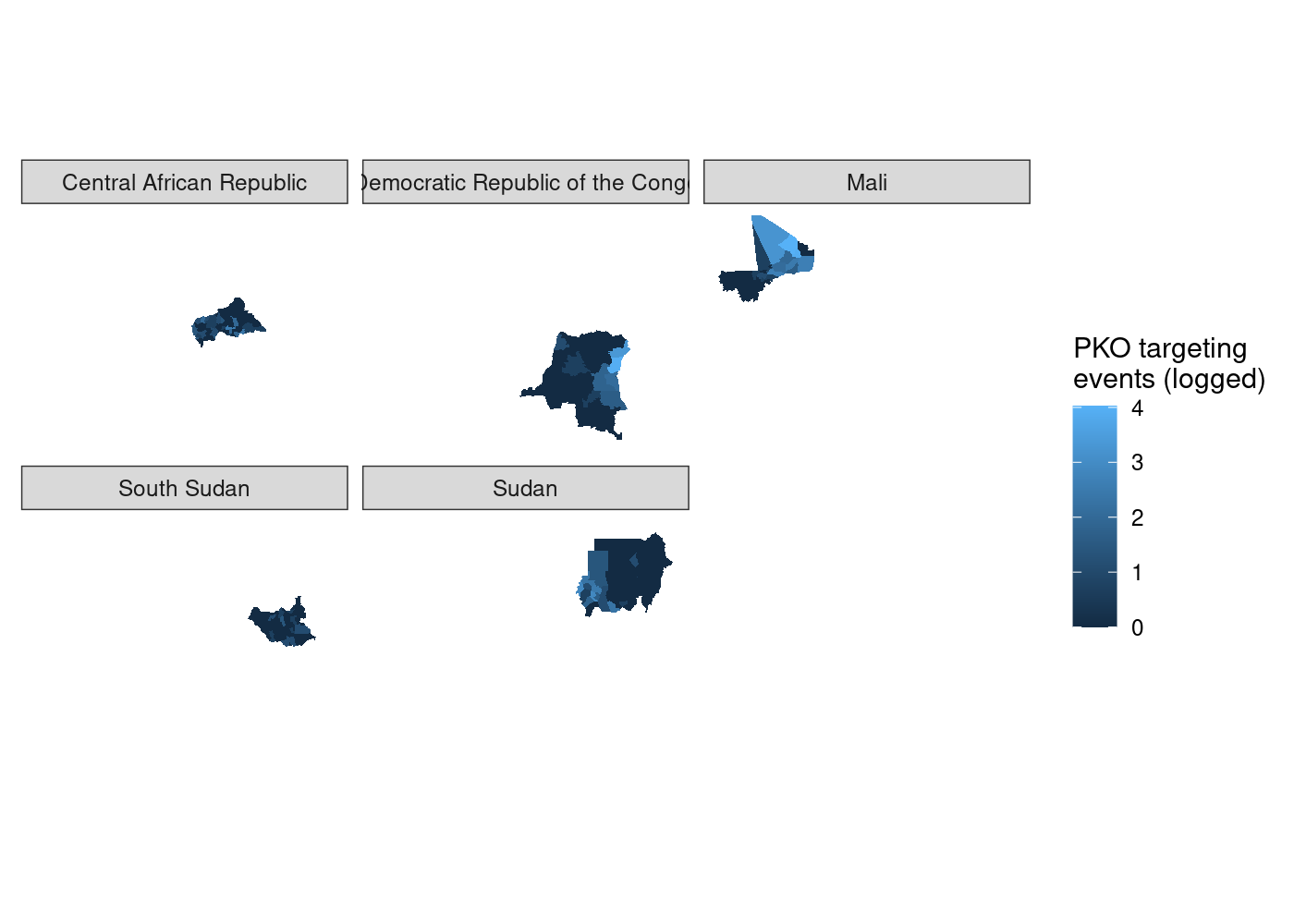
<code class="language-plaintext highlighter-rouge">facet_wrap()</code> call to our <code class="language-plaintext highlighter-rouge">ggplot2</code> code, and tell it to split by our
country name variable, <code class="language-plaintext highlighter-rouge">NAME_0</code>:</p>

<div class="language-r highlighter-rouge"><div class="highlight"><pre class="highlight"><code><span class="n">adm</span><span class="w"> </span><span class="o">%&gt;%</span><span class="w"> 
  </span><span class="n">st_join</span><span class="p">(</span><span class="n">acled</span><span class="p">)</span><span class="w"> </span><span class="o">%&gt;%</span><span class="w"> 
  </span><span class="n">group_by</span><span class="p">(</span><span class="n">NAME_0</span><span class="p">,</span><span class="w"> </span><span class="n">NAME_1</span><span class="p">,</span><span class="w"> </span><span class="n">NAME_2</span><span class="p">)</span><span class="w"> </span><span class="o">%&gt;%</span><span class="w"> 
  </span><span class="n">summarize</span><span class="p">(</span><span class="n">attacks</span><span class="w"> </span><span class="o">=</span><span class="w"> </span><span class="n">log1p</span><span class="p">(</span><span class="nf">sum</span><span class="p">(</span><span class="o">!</span><span class="nf">is.na</span><span class="p">(</span><span class="n">event_id_cnty</span><span class="p">))))</span><span class="w"> </span><span class="o">%&gt;%</span><span class="w"> 
  </span><span class="n">ggplot</span><span class="p">(</span><span class="n">aes</span><span class="p">(</span><span class="n">fill</span><span class="w"> </span><span class="o">=</span><span class="w"> </span><span class="n">attacks</span><span class="p">))</span><span class="w"> </span><span class="o">+</span><span class="w">
  </span><span class="n">geom_sf</span><span class="p">(</span><span class="n">lwd</span><span class="w"> </span><span class="o">=</span><span class="w"> </span><span class="kc">NA</span><span class="p">)</span><span class="w"> </span><span class="o">+</span><span class="w">
  </span><span class="n">scale_fill_continuous</span><span class="p">(</span><span class="n">name</span><span class="w"> </span><span class="o">=</span><span class="w"> </span><span class="s1">'PKO targeting\nevents (logged)'</span><span class="p">)</span><span class="w"> </span><span class="o">+</span><span class="w">
  </span><span class="n">facet_wrap</span><span class="p">(</span><span class="o">~</span><span class="w"> </span><span class="n">NAME_0</span><span class="p">)</span><span class="w"> </span><span class="o">+</span><span class="w">
  </span><span class="n">theme_rw</span><span class="p">()</span><span class="w"> </span><span class="o">+</span><span class="w">
  </span><span class="n">theme</span><span class="p">(</span><span class="n">axis.text</span><span class="w"> </span><span class="o">=</span><span class="w"> </span><span class="n">element_blank</span><span class="p">(),</span><span class="w">
        </span><span class="n">axis.ticks</span><span class="w"> </span><span class="o">=</span><span class="w"> </span><span class="n">element_blank</span><span class="p">())</span><span class="w">
</span></code></pre></div></div>

<p><img src="/images/posts/geom-sf-facet/facets_raw-1.png" style="display: block; margin: auto;" />
We’ve got facets, but everything is still clearly on the same scale.
let’s set <code class="language-plaintext highlighter-rouge">scales = 'free'</code> in our call to <code class="language-plaintext highlighter-rouge">facet_wrap()</code> to try and fix
that.</p>

<div class="language-r highlighter-rouge"><div class="highlight"><pre class="highlight"><code><span class="n">st_join</span><span class="p">(</span><span class="n">adm</span><span class="p">,</span><span class="w"> </span><span class="n">acled</span><span class="p">)</span><span class="w"> </span><span class="o">%&gt;%</span><span class="w"> 
  </span><span class="n">group_by</span><span class="p">(</span><span class="n">NAME_0</span><span class="p">,</span><span class="w"> </span><span class="n">NAME_1</span><span class="p">,</span><span class="w"> </span><span class="n">NAME_2</span><span class="p">)</span><span class="w"> </span><span class="o">%&gt;%</span><span class="w"> 
  </span><span class="n">summarize</span><span class="p">(</span><span class="n">attacks</span><span class="w"> </span><span class="o">=</span><span class="w"> </span><span class="n">log1p</span><span class="p">(</span><span class="nf">sum</span><span class="p">(</span><span class="o">!</span><span class="nf">is.na</span><span class="p">(</span><span class="n">event_id_cnty</span><span class="p">))))</span><span class="w"> </span><span class="o">%&gt;%</span><span class="w"> 
  </span><span class="n">ggplot</span><span class="p">(</span><span class="n">aes</span><span class="p">(</span><span class="n">fill</span><span class="w"> </span><span class="o">=</span><span class="w"> </span><span class="n">attacks</span><span class="p">))</span><span class="w"> </span><span class="o">+</span><span class="w">
  </span><span class="n">geom_sf</span><span class="p">(</span><span class="n">lwd</span><span class="w"> </span><span class="o">=</span><span class="w"> </span><span class="kc">NA</span><span class="p">)</span><span class="w"> </span><span class="o">+</span><span class="w">
  </span><span class="n">scale_fill_continuous</span><span class="p">(</span><span class="n">name</span><span class="w"> </span><span class="o">=</span><span class="w"> </span><span class="s1">'PKO targeting\nevents (logged)'</span><span class="p">)</span><span class="w"> </span><span class="o">+</span><span class="w">
  </span><span class="n">facet_wrap</span><span class="p">(</span><span class="o">~</span><span class="w"> </span><span class="n">NAME_0</span><span class="p">,</span><span class="w"> </span><span class="n">scales</span><span class="w"> </span><span class="o">=</span><span class="w"> </span><span class="s1">'free'</span><span class="p">)</span><span class="w"> </span><span class="o">+</span><span class="w">
  </span><span class="n">theme_rw</span><span class="p">()</span><span class="w"> </span><span class="o">+</span><span class="w">
  </span><span class="n">theme</span><span class="p">(</span><span class="n">axis.text</span><span class="w"> </span><span class="o">=</span><span class="w"> </span><span class="n">element_blank</span><span class="p">(),</span><span class="w">
        </span><span class="n">axis.ticks</span><span class="w"> </span><span class="o">=</span><span class="w"> </span><span class="n">element_blank</span><span class="p">())</span><span class="w">
</span></code></pre></div></div>

<div class="language-plaintext highlighter-rouge"><div class="highlight"><pre class="highlight"><code>## Error: coord_sf doesn't support free scales
</code></pre></div></div>

<p>And we get an error. It turns out the the <code class="language-plaintext highlighter-rouge">ggplot2</code> codebase <a href="https://github.com/tidyverse/ggplot2/issues/2651#issuecomment-391011703">assumes
that it can maniulate axes independently of one
another</a>.
This is very much not the case with geographic data where a meter
vertically needs to equal a meter horizontally, so <code class="language-plaintext highlighter-rouge">coord_sf()</code> locks
the axes in much the same manner as <code class="language-plaintext highlighter-rouge">coord_fixed()</code>.<sup id="fnref:2" role="doc-noteref"><a href="#fn:2" class="footnote" rel="footnote">2</a></sup> To try and get
around the limitations from <code class="language-plaintext highlighter-rouge">ggplot2</code>’s non-spatial origins, I turned to
a package written from the ground up for plotting spatial data.</p>

<h1 id="second-attempt-tmap">Second attempt: <code class="language-plaintext highlighter-rouge">tmap</code></h1>

<p>My googling led me to this <a href="https://stackoverflow.com/a/47679646">Stack Overflow
answer</a> extolling the virtue of
the <code class="language-plaintext highlighter-rouge">tmap</code> package.<sup id="fnref:3" role="doc-noteref"><a href="#fn:3" class="footnote" rel="footnote">3</a></sup> <a href="https://mtennekes.github.io/tmap/"><code class="language-plaintext highlighter-rouge">tmap</code></a> is a
package for drawing thematic maps from <code class="language-plaintext highlighter-rouge">sf</code> objects using a syntax very
similar to <code class="language-plaintext highlighter-rouge">ggplot2</code>. We can reuse the same data wrangling code and as
before pipe it into our plotting function, which this time is
<code class="language-plaintext highlighter-rouge">tm_shape()</code>. We then add a call to <code class="language-plaintext highlighter-rouge">tm_polygons()</code> to get our colored
features and <code class="language-plaintext highlighter-rouge">tm_facet()</code> to split them apart. Note that unlike
<code class="language-plaintext highlighter-rouge">ggplot2</code>, we need to quote the names of variables in <code class="language-plaintext highlighter-rouge">tmap</code> functions:</p>

<div class="language-r highlighter-rouge"><div class="highlight"><pre class="highlight"><code><span class="n">st_join</span><span class="p">(</span><span class="n">adm</span><span class="p">,</span><span class="w"> </span><span class="n">acled</span><span class="p">)</span><span class="w"> </span><span class="o">%&gt;%</span><span class="w"> 
  </span><span class="n">group_by</span><span class="p">(</span><span class="n">NAME_0</span><span class="p">,</span><span class="w"> </span><span class="n">NAME_1</span><span class="p">,</span><span class="w"> </span><span class="n">NAME_2</span><span class="p">)</span><span class="w"> </span><span class="o">%&gt;%</span><span class="w"> 
  </span><span class="n">summarize</span><span class="p">(</span><span class="n">attacks</span><span class="w"> </span><span class="o">=</span><span class="w"> </span><span class="n">log1p</span><span class="p">(</span><span class="nf">sum</span><span class="p">(</span><span class="o">!</span><span class="nf">is.na</span><span class="p">(</span><span class="n">event_id_cnty</span><span class="p">))))</span><span class="w"> </span><span class="o">%&gt;%</span><span class="w"> 
  </span><span class="n">tm_shape</span><span class="p">()</span><span class="w"> </span><span class="o">+</span><span class="w">
  </span><span class="n">tm_polygons</span><span class="p">(</span><span class="s1">'attacks'</span><span class="p">,</span><span class="w"> </span><span class="n">title</span><span class="w"> </span><span class="o">=</span><span class="w"> </span><span class="s1">'PKO targeting\nevents (logged)'</span><span class="p">)</span><span class="w"> </span><span class="o">+</span><span class="w">
  </span><span class="n">tm_facets</span><span class="p">(</span><span class="s1">'NAME_0'</span><span class="p">)</span><span class="w">
</span></code></pre></div></div>

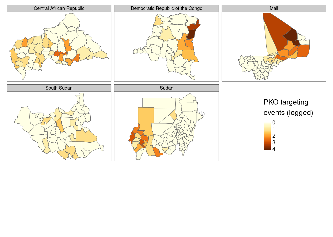
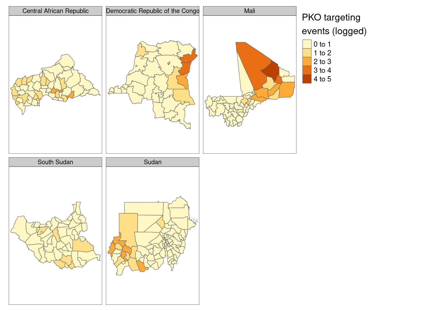
<p><img src="/images/posts/geom-sf-facet/tmap_basic-1.png" style="display: block; margin: auto;" /></p>

<p>Much better so far! However, notice that <code class="language-plaintext highlighter-rouge">tmap</code> defaults to assuming
that our <code class="language-plaintext highlighter-rouge">attacks</code> variable is discrete. We’ll need to tell it that it’s
continuous. And what if we moved that legend down to the bottom right to
get rid of the wasted space currently there?</p>

<div class="language-r highlighter-rouge"><div class="highlight"><pre class="highlight"><code><span class="n">adm</span><span class="w"> </span><span class="o">%&gt;%</span><span class="w"> 
  </span><span class="n">st_join</span><span class="p">(</span><span class="n">acled</span><span class="p">)</span><span class="w"> </span><span class="o">%&gt;%</span><span class="w"> 
  </span><span class="n">group_by</span><span class="p">(</span><span class="n">NAME_0</span><span class="p">,</span><span class="w"> </span><span class="n">NAME_1</span><span class="p">,</span><span class="w"> </span><span class="n">NAME_2</span><span class="p">)</span><span class="w"> </span><span class="o">%&gt;%</span><span class="w"> 
  </span><span class="n">summarize</span><span class="p">(</span><span class="n">attacks</span><span class="w"> </span><span class="o">=</span><span class="w"> </span><span class="n">log1p</span><span class="p">(</span><span class="nf">sum</span><span class="p">(</span><span class="o">!</span><span class="nf">is.na</span><span class="p">(</span><span class="n">event_id_cnty</span><span class="p">))))</span><span class="w"> </span><span class="o">%&gt;%</span><span class="w"> 
  </span><span class="n">tm_shape</span><span class="p">()</span><span class="w"> </span><span class="o">+</span><span class="w">
  </span><span class="n">tm_polygons</span><span class="p">(</span><span class="n">col</span><span class="w"> </span><span class="o">=</span><span class="w"> </span><span class="s1">'attacks'</span><span class="p">,</span><span class="w">
              </span><span class="n">title</span><span class="w"> </span><span class="o">=</span><span class="w"> </span><span class="s1">'PKO targeting\nevents (logged)'</span><span class="p">,</span><span class="w">
              </span><span class="n">style</span><span class="w"> </span><span class="o">=</span><span class="w"> </span><span class="s1">'cont'</span><span class="p">)</span><span class="w"> </span><span class="o">+</span><span class="w">                  </span><span class="c1"># continuous variable</span><span class="w">
  </span><span class="n">tm_facets</span><span class="p">(</span><span class="s1">'NAME_0'</span><span class="p">)</span><span class="w"> </span><span class="o">+</span><span class="w">
  </span><span class="n">tm_layout</span><span class="p">(</span><span class="n">legend.outside.position</span><span class="w"> </span><span class="o">=</span><span class="w">  </span><span class="s2">"bottom"</span><span class="p">,</span><span class="w"> </span><span class="c1"># legend outside below</span><span class="w">
            </span><span class="n">legend.position</span><span class="w"> </span><span class="o">=</span><span class="w"> </span><span class="nf">c</span><span class="p">(</span><span class="m">.8</span><span class="p">,</span><span class="w"> </span><span class="m">1.1</span><span class="p">))</span><span class="w">        </span><span class="c1"># manually position legend</span><span class="w">
</span></code></pre></div></div>

<p><img src="/images/posts/geom-sf-facet/tmap_tweaked-1.png" style="display: block; margin: auto;" /></p>

<p>This is…<em>fine</em>. You’ll notice that there’s a lot of white space at the
bottom of the plot, which I still haven’t figured out how to eliminate,
and I personally prefer the color palette options available in
<code class="language-plaintext highlighter-rouge">ggplot2</code>. Finally, there’s not much control over the legend compared to
what you get with <code class="language-plaintext highlighter-rouge">ggplot2</code>, so let’s head back there and try to come at
this problem from a different direction.</p>

<h1 id="third-attempt-cowplot">Third attempt: <code class="language-plaintext highlighter-rouge">cowplot</code></h1>

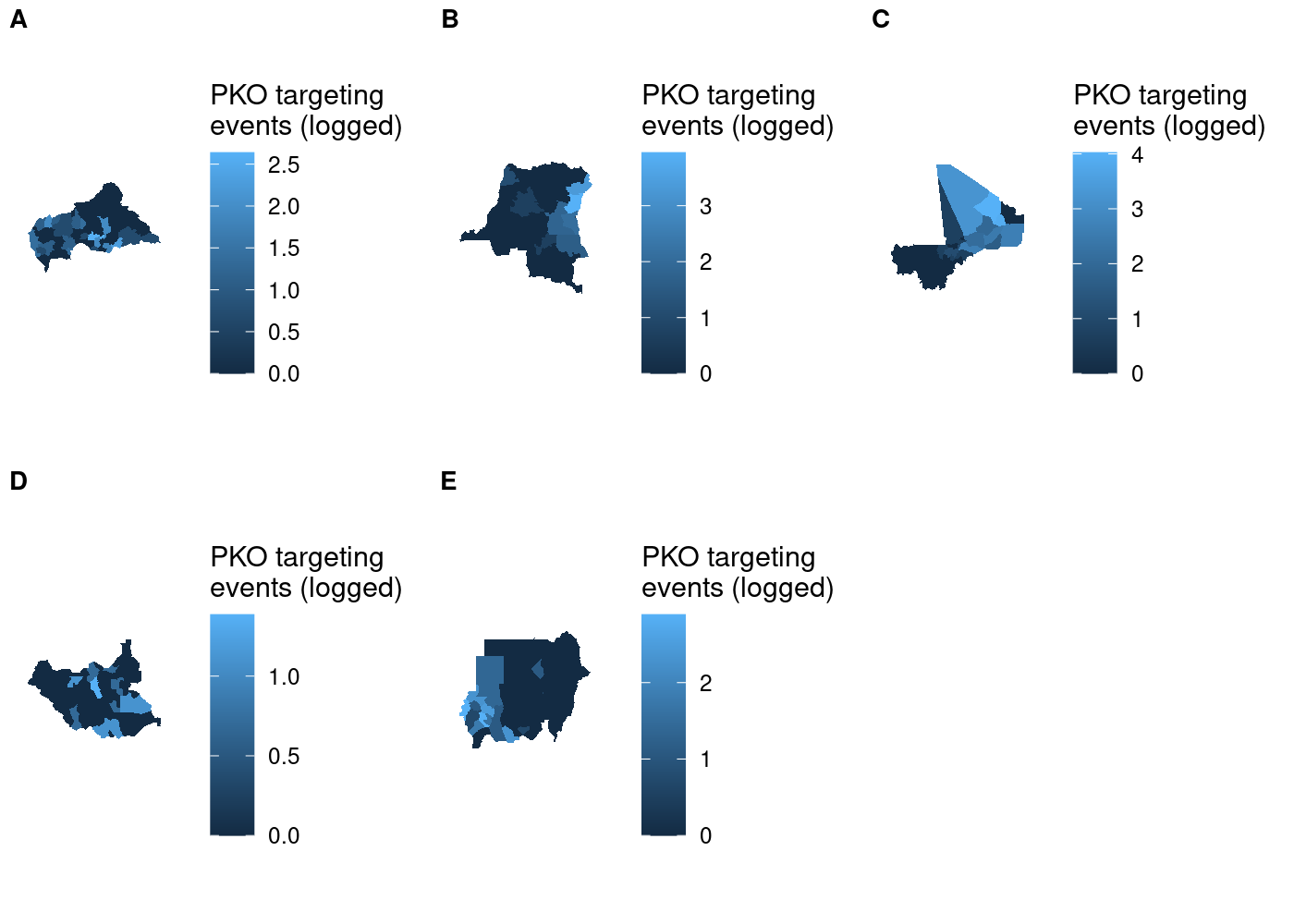
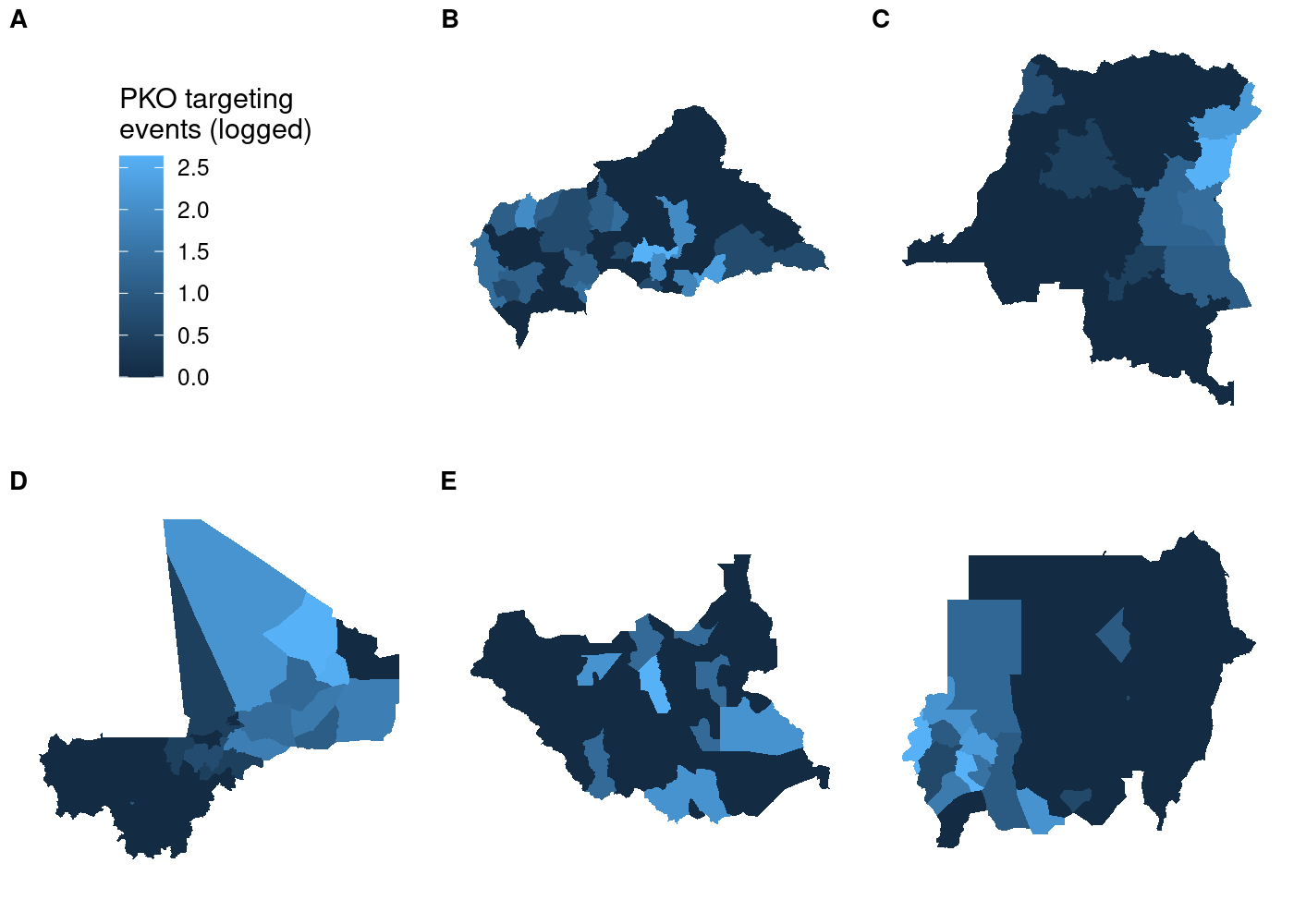
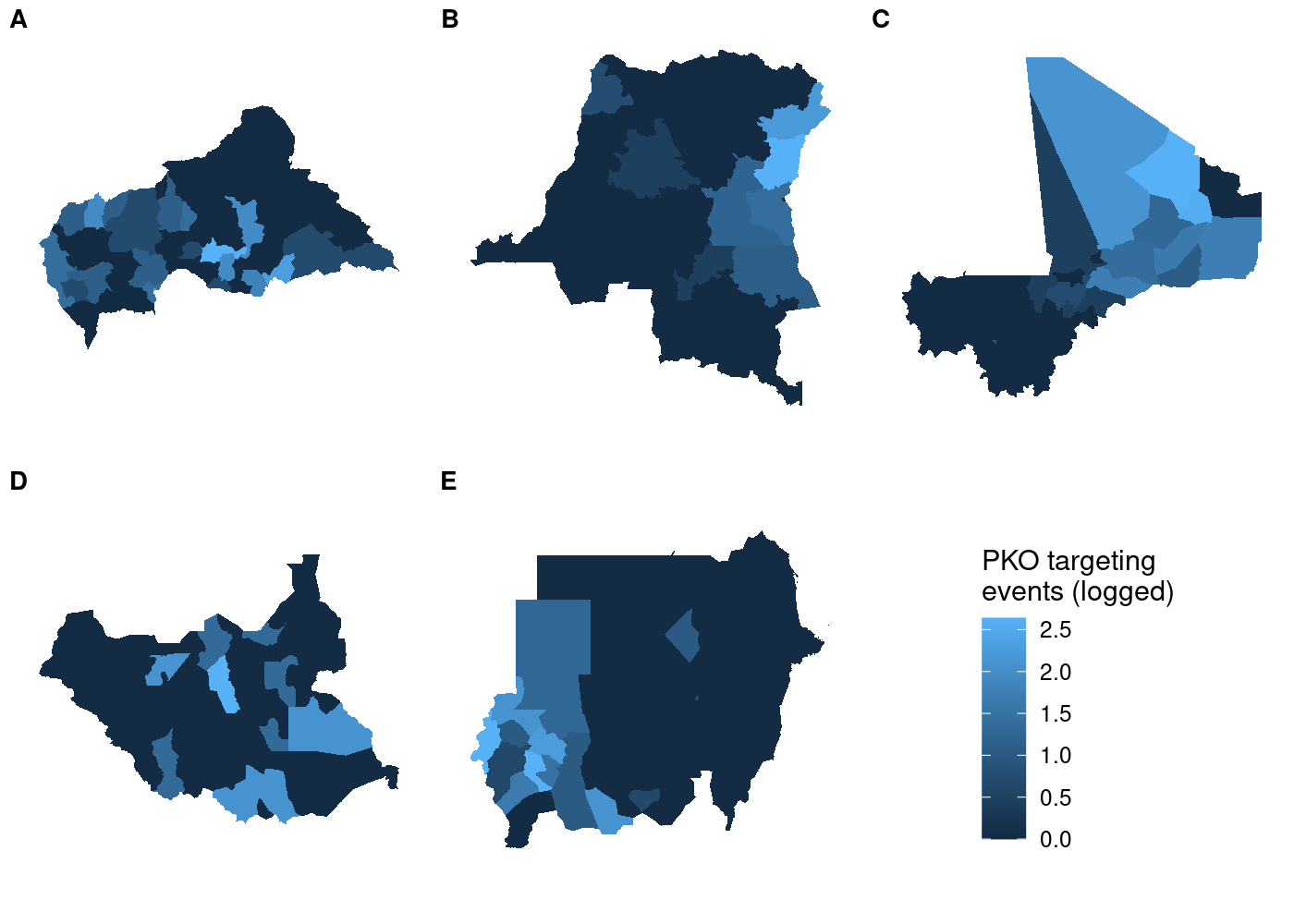
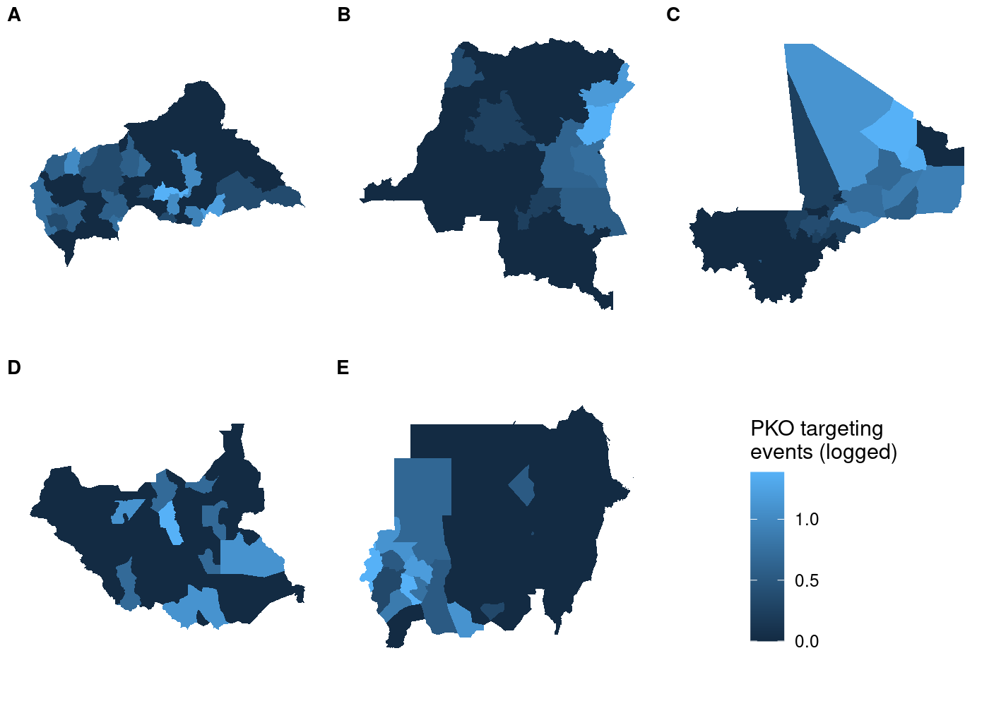
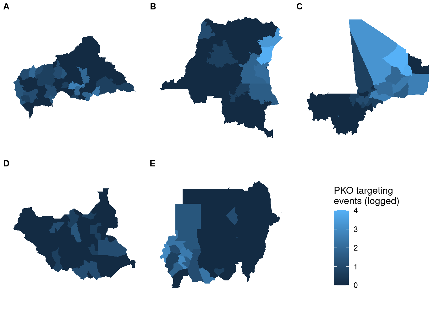
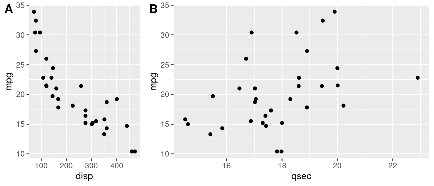
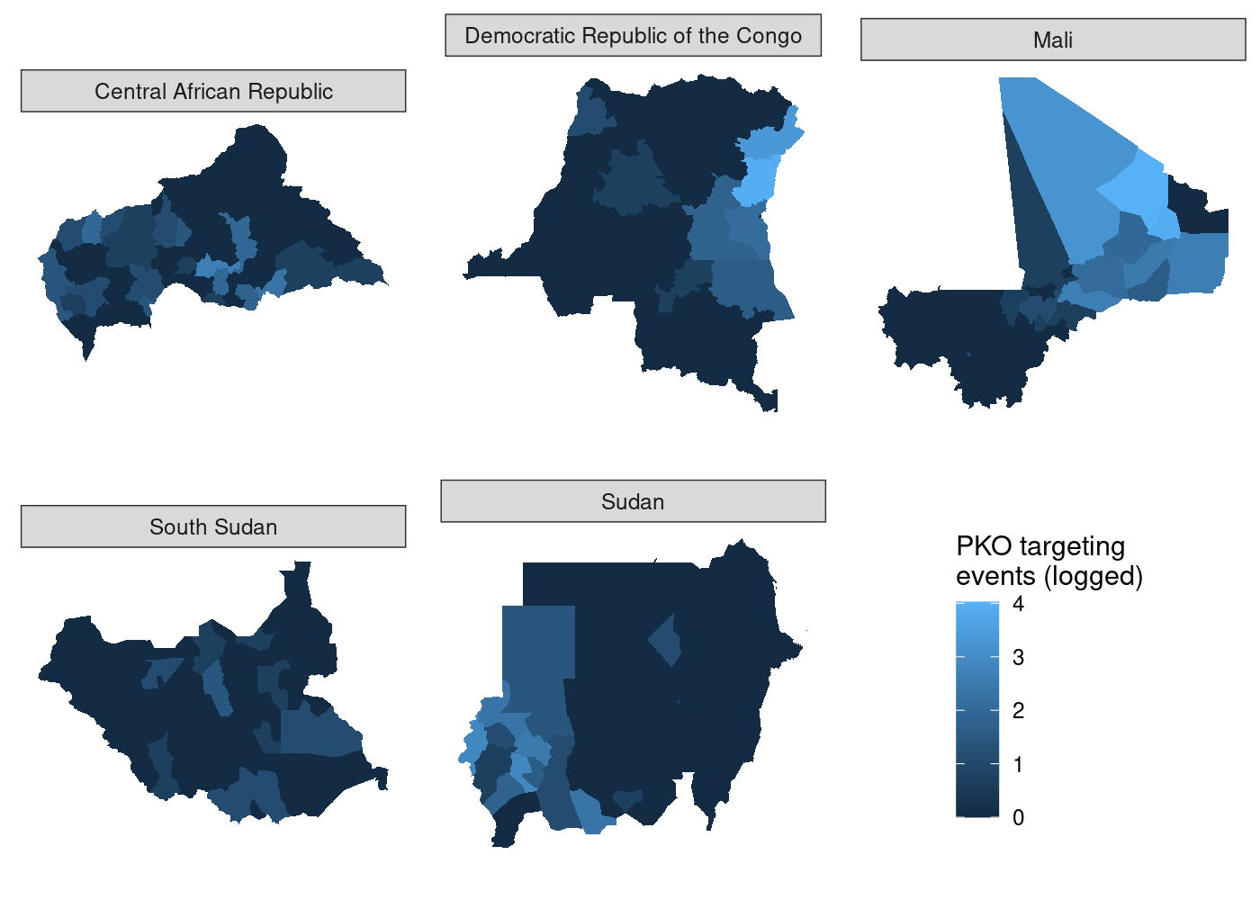
<p>While we’re still using <code class="language-plaintext highlighter-rouge">ggplot2</code> to make individual plots, we need some
way to combine them into a final plot. We can rely on the <code class="language-plaintext highlighter-rouge">plot_grid()</code>
function in the <code class="language-plaintext highlighter-rouge">cowplot</code> library for that.<sup id="fnref:4" role="doc-noteref"><a href="#fn:4" class="footnote" rel="footnote">4</a></sup> We need to create five
subplots, which we could do manually, but let’s do it programmatically
because at some point you may need to do this for 27 different
countries. The best way to store our five subplots is in a list, because
lists in R can contain any type of R objects as their elements.<sup id="fnref:5" role="doc-noteref"><a href="#fn:5" class="footnote" rel="footnote">5</a></sup> I’m
going to use the <code class="language-plaintext highlighter-rouge">map()</code> function from the <code class="language-plaintext highlighter-rouge">purrr</code> package to accomplish
this, but you could also use <code class="language-plaintext highlighter-rouge">lapply()</code>. <code class="language-plaintext highlighter-rouge">map()</code> takes a list as its
first argument, <code class="language-plaintext highlighter-rouge">.x</code> and a function as its second, <code class="language-plaintext highlighter-rouge">.f</code>. To see how map
works, look at the following example:</p>

<div class="language-r highlighter-rouge"><div class="highlight"><pre class="highlight"><code><span class="n">map</span><span class="p">(</span><span class="m">1</span><span class="o">:</span><span class="m">3</span><span class="p">,</span><span class="w"> </span><span class="n">sample</span><span class="p">)</span><span class="w">
</span></code></pre></div></div>

<div class="language-plaintext highlighter-rouge"><div class="highlight"><pre class="highlight"><code>## [[1]]
## [1] 1
## 
## [[2]]
## [1] 1 2
## 
## [[3]]
## [1] 2 3 1
</code></pre></div></div>

<p><code class="language-plaintext highlighter-rouge">map()</code> returns a list of length 3 because our input <code class="language-plaintext highlighter-rouge">.x</code> was a vector
of length three, and it applies the function <code class="language-plaintext highlighter-rouge">.f</code> to each element of
<code class="language-plaintext highlighter-rouge">.x</code>. I’m going to use an <a href="http://adv-r.had.co.nz/Functional-programming.html#anonymous-functions">anonymous
function</a>
to filter <code class="language-plaintext highlighter-rouge">adm</code> to only contain ADM2s from one country at a time, then
create our subplots separately like we did together above:</p>

<div class="language-r highlighter-rouge"><div class="highlight"><pre class="highlight"><code><span class="n">pko_countries</span><span class="w"> </span><span class="o">&lt;-</span><span class="w"> </span><span class="nf">c</span><span class="p">(</span><span class="s1">'Central African Republic'</span><span class="p">,</span><span class="w"> </span><span class="s1">'Democratic Republic of the Congo'</span><span class="p">,</span><span class="w">
                   </span><span class="s1">'Mali'</span><span class="p">,</span><span class="w"> </span><span class="s1">'South Sudan'</span><span class="p">,</span><span class="w"> </span><span class="s1">'Sudan'</span><span class="p">)</span><span class="w">

</span><span class="c1">## create maps in separate plots, force common scale between them</span><span class="w">
</span><span class="n">maps</span><span class="w"> </span><span class="o">&lt;-</span><span class="w"> </span><span class="n">map</span><span class="p">(</span><span class="n">.x</span><span class="w"> </span><span class="o">=</span><span class="w"> </span><span class="n">pko_countries</span><span class="p">,</span><span class="w"> 
            </span><span class="n">.f</span><span class="w"> </span><span class="o">=</span><span class="w"> </span><span class="k">function</span><span class="p">(</span><span class="n">x</span><span class="p">)</span><span class="w"> </span><span class="n">adm</span><span class="w"> </span><span class="o">%&gt;%</span><span class="w"> 
              </span><span class="n">filter</span><span class="p">(</span><span class="n">NAME_0</span><span class="w"> </span><span class="o">==</span><span class="w"> </span><span class="n">x</span><span class="p">)</span><span class="w"> </span><span class="o">%&gt;%</span><span class="w"> 
              </span><span class="n">st_join</span><span class="p">(</span><span class="n">acled</span><span class="p">)</span><span class="w"> </span><span class="o">%&gt;%</span><span class="w"> 
              </span><span class="n">group_by</span><span class="p">(</span><span class="n">NAME_0</span><span class="p">,</span><span class="w"> </span><span class="n">NAME_1</span><span class="p">,</span><span class="w"> </span><span class="n">NAME_2</span><span class="p">)</span><span class="w"> </span><span class="o">%&gt;%</span><span class="w"> 
              </span><span class="n">summarize</span><span class="p">(</span><span class="n">attacks</span><span class="w"> </span><span class="o">=</span><span class="w"> </span><span class="n">log1p</span><span class="p">(</span><span class="nf">sum</span><span class="p">(</span><span class="o">!</span><span class="nf">is.na</span><span class="p">(</span><span class="n">event_id_cnty</span><span class="p">))))</span><span class="w"> </span><span class="o">%&gt;%</span><span class="w"> 
              </span><span class="n">ggplot</span><span class="p">(</span><span class="n">aes</span><span class="p">(</span><span class="n">fill</span><span class="w"> </span><span class="o">=</span><span class="w"> </span><span class="n">attacks</span><span class="p">))</span><span class="w"> </span><span class="o">+</span><span class="w">
              </span><span class="n">geom_sf</span><span class="p">(</span><span class="n">lwd</span><span class="w"> </span><span class="o">=</span><span class="w"> </span><span class="kc">NA</span><span class="p">)</span><span class="w"> </span><span class="o">+</span><span class="w">
              </span><span class="n">scale_fill_continuous</span><span class="p">(</span><span class="n">name</span><span class="w"> </span><span class="o">=</span><span class="w"> </span><span class="s1">'PKO targeting\nevents (logged)'</span><span class="p">)</span><span class="w"> </span><span class="o">+</span><span class="w">
              </span><span class="n">theme_rw</span><span class="p">()</span><span class="w"> </span><span class="o">+</span><span class="w">
              </span><span class="n">theme</span><span class="p">(</span><span class="n">axis.text</span><span class="w"> </span><span class="o">=</span><span class="w"> </span><span class="n">element_blank</span><span class="p">(),</span><span class="w">
                    </span><span class="n">axis.ticks</span><span class="w"> </span><span class="o">=</span><span class="w"> </span><span class="n">element_blank</span><span class="p">()))</span><span class="w">
</span></code></pre></div></div>

<p>We can either supply each individual subplot to <code class="language-plaintext highlighter-rouge">plot_grid()</code>
separately, or we can use the <code class="language-plaintext highlighter-rouge">plotlist</code> argument to pass a list of
plots; good thing we saved them in a list:</p>

<div class="language-r highlighter-rouge"><div class="highlight"><pre class="highlight"><code><span class="c1">## use COWplot to combine and add single legend</span><span class="w">
</span><span class="n">plot_grid</span><span class="p">(</span><span class="n">plotlist</span><span class="w"> </span><span class="o">=</span><span class="w"> </span><span class="n">maps</span><span class="p">,</span><span class="w"> </span><span class="n">labels</span><span class="w"> </span><span class="o">=</span><span class="w"> </span><span class="nb">LETTERS</span><span class="p">[</span><span class="m">1</span><span class="o">:</span><span class="m">5</span><span class="p">],</span><span class="w"> </span><span class="n">label_size</span><span class="w"> </span><span class="o">=</span><span class="w"> </span><span class="m">10</span><span class="p">,</span><span class="w"> </span><span class="n">nrow</span><span class="w"> </span><span class="o">=</span><span class="w"> </span><span class="m">2</span><span class="p">)</span><span class="w">
</span></code></pre></div></div>

<p><img src="/images/posts/geom-sf-facet/individual_legends-1.png" style="display: block; margin: auto;" /></p>

<p>I tried using the name of each country as the subplot label, but because
<a href="https://github.com/wilkelab/cowplot/issues/32#issuecomment-198428848">label positioning is relative to the width of
labels</a>
it was impossible to get them all nicely left-aligned. As a result, I
had to settle on using letters to label the subplots and then
identifying them in the figure caption in text. As you’ll see
<a href="#bonus-still-to-solve">later</a>, there’s no perfect way of accomplishing
this and you’ll have to make a trade-off somewhere.</p>

<p>Setting aside that compromise, there’s still one issue with this plot
that we can fix. We’re measuring the same thing (attacks on UN
peacekeeping personnel) in all five choropleths, so there’s no need for
five separate scales.</p>

<h2 id="shared-legend">Shared legend</h2>

<p>The <code class="language-plaintext highlighter-rouge">cowplot</code>
<a href="https://wilkelab.org/cowplot/articles/shared_legends.html">documentation</a>
demonstrates how to use the <code class="language-plaintext highlighter-rouge">get_legend()</code> function to extract the
legend from one of the subplots and then add it as another element to
<code class="language-plaintext highlighter-rouge">plot_grid()</code>, placing it in the bottom right like we sort of managed to
do with <code class="language-plaintext highlighter-rouge">tmap</code>. However, we need to add
<code class="language-plaintext highlighter-rouge">theme(legend.position = 'none')</code> to the ggplot call for each subplot,
otherwise we’ll just end up with six legends. That means we need to
apply to each element of our list of maps, which means it’s another job
that <code class="language-plaintext highlighter-rouge">map()</code> is perfect for! We’ll use <code class="language-plaintext highlighter-rouge">map()</code> to take each subplot in
<code class="language-plaintext highlighter-rouge">maps</code> and remove the legend from it, then use <code class="language-plaintext highlighter-rouge">get_legend()</code> to add a
legend in the bottom right.</p>

<div class="language-r highlighter-rouge"><div class="highlight"><pre class="highlight"><code><span class="c1">## use COWplot to combine and add single legend</span><span class="w">
</span><span class="n">plot_grid</span><span class="p">(</span><span class="n">plotlist</span><span class="w"> </span><span class="o">=</span><span class="w"> </span><span class="nf">c</span><span class="p">(</span><span class="n">map</span><span class="p">(</span><span class="n">.x</span><span class="w"> </span><span class="o">=</span><span class="w"> </span><span class="n">maps</span><span class="p">,</span><span class="w">
                           </span><span class="n">.f</span><span class="w"> </span><span class="o">=</span><span class="w"> </span><span class="k">function</span><span class="p">(</span><span class="n">x</span><span class="p">)</span><span class="w"> </span><span class="n">x</span><span class="w"> </span><span class="o">+</span><span class="w"> </span><span class="n">theme</span><span class="p">(</span><span class="n">legend.position</span><span class="w"> </span><span class="o">=</span><span class="w"> </span><span class="s1">'none'</span><span class="p">))),</span><span class="w">
          </span><span class="n">get_legend</span><span class="p">(</span><span class="n">maps</span><span class="p">[[</span><span class="m">1</span><span class="p">]]),</span><span class="w">
          </span><span class="n">labels</span><span class="w"> </span><span class="o">=</span><span class="w"> </span><span class="nb">LETTERS</span><span class="p">[</span><span class="m">1</span><span class="o">:</span><span class="m">5</span><span class="p">],</span><span class="w"> </span><span class="n">label_size</span><span class="w"> </span><span class="o">=</span><span class="w"> </span><span class="m">10</span><span class="p">,</span><span class="w"> </span><span class="n">nrow</span><span class="w"> </span><span class="o">=</span><span class="w"> </span><span class="m">2</span><span class="p">)</span><span class="w">
</span></code></pre></div></div>

<p><img src="/images/posts/geom-sf-facet/shared_legend_missing-1.png" style="display: block; margin: auto;" />
This doesn’t look right! We told <code class="language-plaintext highlighter-rouge">plot_grid()</code> to start with our maps,
so why is the legend the first thing in the plot? If you look closely at
the documentation for <code class="language-plaintext highlighter-rouge">plot_grid()</code>, you’ll see that the <code class="language-plaintext highlighter-rouge">...</code> argument
comes before the <code class="language-plaintext highlighter-rouge">plotlist</code> argument in the function definition. Even
when we specify <code class="language-plaintext highlighter-rouge">plotlist</code> first, the function will add <code class="language-plaintext highlighter-rouge">plotlist</code> after
<code class="language-plaintext highlighter-rouge">...</code>.<sup id="fnref:6" role="doc-noteref"><a href="#fn:6" class="footnote" rel="footnote">6</a></sup> To fix this, all we need to do is concatenate the results of
<code class="language-plaintext highlighter-rouge">get_legend()</code> with the results of our call to <code class="language-plaintext highlighter-rouge">map()</code>. Note that we
need to first transform the former to a list with <code class="language-plaintext highlighter-rouge">list()</code>, otherwise
each element of it will be concatenated separately rather than as a
<code class="language-plaintext highlighter-rouge">grob</code> object:</p>

<div class="language-r highlighter-rouge"><div class="highlight"><pre class="highlight"><code><span class="c1">## use COWplot to combine and add single legend</span><span class="w">
</span><span class="n">plot_grid</span><span class="p">(</span><span class="n">plotlist</span><span class="w"> </span><span class="o">=</span><span class="w"> </span><span class="nf">c</span><span class="p">(</span><span class="n">map</span><span class="p">(</span><span class="n">.x</span><span class="w"> </span><span class="o">=</span><span class="w"> </span><span class="n">maps</span><span class="p">,</span><span class="w">
                           </span><span class="n">.f</span><span class="w"> </span><span class="o">=</span><span class="w"> </span><span class="k">function</span><span class="p">(</span><span class="n">x</span><span class="p">)</span><span class="w"> </span><span class="n">x</span><span class="w"> </span><span class="o">+</span><span class="w"> </span><span class="n">theme</span><span class="p">(</span><span class="n">legend.position</span><span class="w"> </span><span class="o">=</span><span class="w"> </span><span class="s1">'none'</span><span class="p">)),</span><span class="w">
                       </span><span class="nf">list</span><span class="p">(</span><span class="n">get_legend</span><span class="p">(</span><span class="n">maps</span><span class="p">[[</span><span class="m">1</span><span class="p">]]))),</span><span class="w">
          </span><span class="n">labels</span><span class="w"> </span><span class="o">=</span><span class="w"> </span><span class="nb">LETTERS</span><span class="p">[</span><span class="m">1</span><span class="o">:</span><span class="m">5</span><span class="p">],</span><span class="w">
          </span><span class="n">label_size</span><span class="w"> </span><span class="o">=</span><span class="w"> </span><span class="m">10</span><span class="p">,</span><span class="w">
          </span><span class="n">nrow</span><span class="w"> </span><span class="o">=</span><span class="w"> </span><span class="m">2</span><span class="p">)</span><span class="w">
</span></code></pre></div></div>

<p><img src="/images/posts/geom-sf-facet/shared_legend_wrong-1.png" style="display: block; margin: auto;" /></p>

<p>So far so good. But if we try using a different map in our call to
<code class="language-plaintext highlighter-rouge">get_legend()</code>, things get weird:</p>

<div class="language-r highlighter-rouge"><div class="highlight"><pre class="highlight"><code><span class="c1">## use COWplot to combine and add single legend</span><span class="w">
</span><span class="n">plot_grid</span><span class="p">(</span><span class="n">plotlist</span><span class="w"> </span><span class="o">=</span><span class="w"> </span><span class="nf">c</span><span class="p">(</span><span class="n">map</span><span class="p">(</span><span class="n">.x</span><span class="w"> </span><span class="o">=</span><span class="w"> </span><span class="n">maps</span><span class="p">,</span><span class="w">
                           </span><span class="n">.f</span><span class="w"> </span><span class="o">=</span><span class="w"> </span><span class="k">function</span><span class="p">(</span><span class="n">x</span><span class="p">)</span><span class="w"> </span><span class="n">x</span><span class="w"> </span><span class="o">+</span><span class="w"> </span><span class="n">theme</span><span class="p">(</span><span class="n">legend.position</span><span class="w"> </span><span class="o">=</span><span class="w"> </span><span class="s1">'none'</span><span class="p">)),</span><span class="w">
                       </span><span class="nf">list</span><span class="p">(</span><span class="n">get_legend</span><span class="p">(</span><span class="n">maps</span><span class="p">[[</span><span class="m">4</span><span class="p">]]))),</span><span class="w">
          </span><span class="n">labels</span><span class="w"> </span><span class="o">=</span><span class="w"> </span><span class="nb">LETTERS</span><span class="p">[</span><span class="m">1</span><span class="o">:</span><span class="m">5</span><span class="p">],</span><span class="w"> </span><span class="n">label_size</span><span class="w"> </span><span class="o">=</span><span class="w"> </span><span class="m">10</span><span class="p">,</span><span class="w"> </span><span class="n">nrow</span><span class="w"> </span><span class="o">=</span><span class="w"> </span><span class="m">2</span><span class="p">)</span><span class="w">
</span></code></pre></div></div>

<p><img src="/images/posts/geom-sf-facet/shared_legend_wrong2-1.png" style="display: block; margin: auto;" />
Each subplot has its own unique legend that’s automatically generated
from the values of <code class="language-plaintext highlighter-rouge">attacks</code> it contains. This is even worse than it
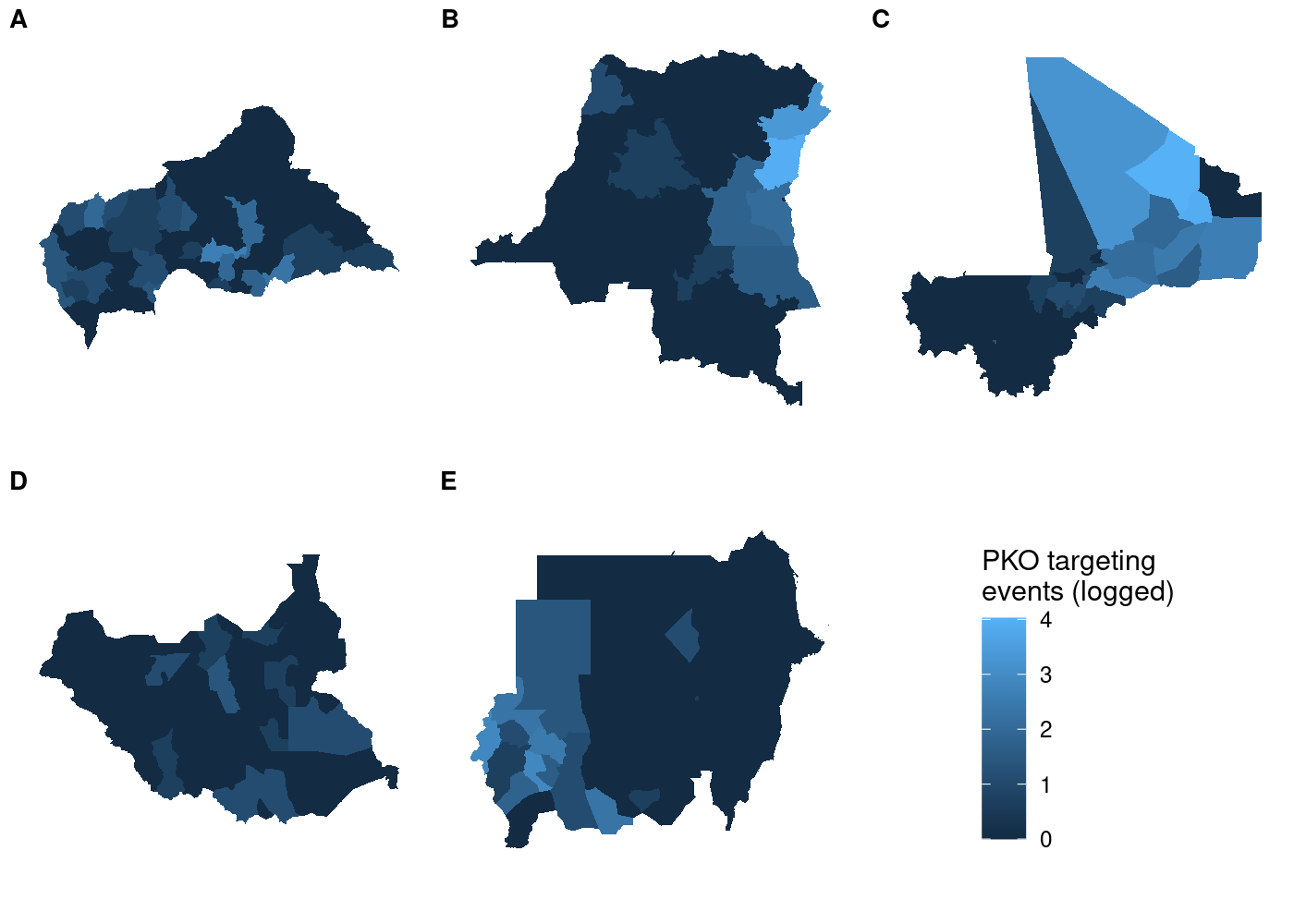
might seem at first glance, because it means that the various subplots
are in no way comparable to one another!</p>

<h2 id="accurate-shared-legend">Accurate shared legend</h2>

<p>To avoid misrepresenting the data, we need to ensure that each subplot
has the same legend. The easiest way to do this is to manually set the
legend for each subplot in our call to <code class="language-plaintext highlighter-rouge">scale_fill_continuous()</code>. Even
though we’re manually setting the bounds of the legend, that doesn’t
mean we have to hard code them. We can use a simpler version of our code
to join attacks to ADM2s and then calculate the highest number of
attacks across <em>all</em> countries in the data. Then we take advantage of
the fact that <code class="language-plaintext highlighter-rouge">scale_fill_continuous()</code> can pass additional parameters
to <code class="language-plaintext highlighter-rouge">continuous_scale()</code> via the <code class="language-plaintext highlighter-rouge">...</code> argument. The <code class="language-plaintext highlighter-rouge">continuous_scale()</code>
function is a low-level function used throughout <code class="language-plaintext highlighter-rouge">ggplot2</code> to construct
continuous scales, and it has a <code class="language-plaintext highlighter-rouge">limits</code> argument that sets the bounds
of the scale. All we have to do is pass the minimum and maximum (logged)
numbers of attacks in the data and we’re in business:</p>

<div class="language-r highlighter-rouge"><div class="highlight"><pre class="highlight"><code><span class="n">st_join</span><span class="p">(</span><span class="n">adm</span><span class="p">,</span><span class="w"> </span><span class="n">acled</span><span class="p">)</span><span class="w"> </span><span class="o">%&gt;%</span><span class="w"> 
  </span><span class="n">st_drop_geometry</span><span class="p">()</span><span class="w"> </span><span class="o">%&gt;%</span><span class="w">   </span><span class="c1"># we don't need a map at the end; drop geometry to speed up</span><span class="w">
  </span><span class="n">group_by</span><span class="p">(</span><span class="n">NAME_0</span><span class="p">,</span><span class="w"> </span><span class="n">NAME_1</span><span class="p">,</span><span class="w"> </span><span class="n">NAME_2</span><span class="p">)</span><span class="w"> </span><span class="o">%&gt;%</span><span class="w"> 
  </span><span class="n">summarize</span><span class="p">(</span><span class="n">attacks</span><span class="w"> </span><span class="o">=</span><span class="w"> </span><span class="n">log1p</span><span class="p">(</span><span class="nf">sum</span><span class="p">(</span><span class="o">!</span><span class="nf">is.na</span><span class="p">(</span><span class="n">event_id_cnty</span><span class="p">))))</span><span class="w"> </span><span class="o">%&gt;%</span><span class="w"> 
  </span><span class="n">pull</span><span class="p">(</span><span class="n">attacks</span><span class="p">)</span><span class="w"> </span><span class="o">%&gt;%</span><span class="w">        </span><span class="c1"># extract attacks variable</span><span class="w">
  </span><span class="nf">range</span><span class="p">()</span><span class="w"> </span><span class="o">-&gt;</span><span class="w"> </span><span class="n">attacks_range</span><span class="w"> </span><span class="c1"># get min and max</span><span class="w">

</span><span class="c1">## create maps in separate plots, force common scale between them</span><span class="w">
</span><span class="n">maps_shared</span><span class="w"> </span><span class="o">&lt;-</span><span class="w"> </span><span class="n">map</span><span class="p">(</span><span class="n">.x</span><span class="w"> </span><span class="o">=</span><span class="w"> </span><span class="n">pko_countries</span><span class="p">,</span><span class="w"> 
                   </span><span class="n">.f</span><span class="w"> </span><span class="o">=</span><span class="w"> </span><span class="k">function</span><span class="p">(</span><span class="n">x</span><span class="p">)</span><span class="w"> </span><span class="n">adm</span><span class="w"> </span><span class="o">%&gt;%</span><span class="w"> 
                     </span><span class="n">filter</span><span class="p">(</span><span class="n">NAME_0</span><span class="w"> </span><span class="o">==</span><span class="w"> </span><span class="n">x</span><span class="p">)</span><span class="w"> </span><span class="o">%&gt;%</span><span class="w"> 
                     </span><span class="n">st_join</span><span class="p">(</span><span class="n">acled</span><span class="p">)</span><span class="w"> </span><span class="o">%&gt;%</span><span class="w"> 
                     </span><span class="n">group_by</span><span class="p">(</span><span class="n">NAME_0</span><span class="p">,</span><span class="w"> </span><span class="n">NAME_1</span><span class="p">,</span><span class="w"> </span><span class="n">NAME_2</span><span class="p">)</span><span class="w"> </span><span class="o">%&gt;%</span><span class="w"> 
                     </span><span class="n">summarize</span><span class="p">(</span><span class="n">attacks</span><span class="w"> </span><span class="o">=</span><span class="w"> </span><span class="n">log1p</span><span class="p">(</span><span class="nf">sum</span><span class="p">(</span><span class="o">!</span><span class="nf">is.na</span><span class="p">(</span><span class="n">event_id_cnty</span><span class="p">))))</span><span class="w"> </span><span class="o">%&gt;%</span><span class="w"> 
                     </span><span class="n">ggplot</span><span class="p">(</span><span class="n">aes</span><span class="p">(</span><span class="n">fill</span><span class="w"> </span><span class="o">=</span><span class="w"> </span><span class="n">attacks</span><span class="p">))</span><span class="w"> </span><span class="o">+</span><span class="w">
                     </span><span class="n">geom_sf</span><span class="p">(</span><span class="n">lwd</span><span class="w"> </span><span class="o">=</span><span class="w"> </span><span class="kc">NA</span><span class="p">)</span><span class="w"> </span><span class="o">+</span><span class="w">
                     </span><span class="n">scale_fill_continuous</span><span class="p">(</span><span class="n">limits</span><span class="w"> </span><span class="o">=</span><span class="w"> </span><span class="n">attacks_range</span><span class="p">,</span><span class="w">
                                           </span><span class="n">name</span><span class="w"> </span><span class="o">=</span><span class="w"> </span><span class="s1">'PKO targeting\nevents (logged)'</span><span class="p">)</span><span class="w"> </span><span class="o">+</span><span class="w">
                     </span><span class="n">theme_rw</span><span class="p">()</span><span class="w"> </span><span class="o">+</span><span class="w">
                     </span><span class="n">theme</span><span class="p">(</span><span class="n">axis.text</span><span class="w"> </span><span class="o">=</span><span class="w"> </span><span class="n">element_blank</span><span class="p">(),</span><span class="w">
                           </span><span class="n">axis.ticks</span><span class="w"> </span><span class="o">=</span><span class="w"> </span><span class="n">element_blank</span><span class="p">()))</span><span class="w">
</span></code></pre></div></div>

<p>Now all that’s left is to use <code class="language-plaintext highlighter-rouge">plot_grid()</code> to put it all together:</p>

<div class="language-r highlighter-rouge"><div class="highlight"><pre class="highlight"><code><span class="c1">## use COWplot to combine and add single legend</span><span class="w">
</span><span class="n">plot_grid</span><span class="p">(</span><span class="n">plotlist</span><span class="w"> </span><span class="o">=</span><span class="w"> </span><span class="nf">c</span><span class="p">(</span><span class="n">map</span><span class="p">(</span><span class="n">.x</span><span class="w"> </span><span class="o">=</span><span class="w"> </span><span class="n">maps_shared</span><span class="p">,</span><span class="w">
                           </span><span class="n">.f</span><span class="w"> </span><span class="o">=</span><span class="w"> </span><span class="k">function</span><span class="p">(</span><span class="n">x</span><span class="p">)</span><span class="w"> </span><span class="n">x</span><span class="w"> </span><span class="o">+</span><span class="w"> </span><span class="n">theme</span><span class="p">(</span><span class="n">legend.position</span><span class="w"> </span><span class="o">=</span><span class="w"> </span><span class="s1">'none'</span><span class="p">)),</span><span class="w">
                       </span><span class="nf">list</span><span class="p">(</span><span class="n">get_legend</span><span class="p">(</span><span class="n">maps_shared</span><span class="p">[[</span><span class="m">1</span><span class="p">]]))),</span><span class="w">
          </span><span class="n">labels</span><span class="w"> </span><span class="o">=</span><span class="w"> </span><span class="nb">LETTERS</span><span class="p">[</span><span class="m">1</span><span class="o">:</span><span class="m">5</span><span class="p">],</span><span class="w"> </span><span class="n">label_size</span><span class="w"> </span><span class="o">=</span><span class="w"> </span><span class="m">10</span><span class="p">,</span><span class="w"> </span><span class="n">nrow</span><span class="w"> </span><span class="o">=</span><span class="w"> </span><span class="m">2</span><span class="p">)</span><span class="w">
</span></code></pre></div></div>

<p><img src="/images/posts/geom-sf-facet/shared_legend_right-1.png" style="display: block; margin: auto;" /></p>

<p>And unlike before, the legend is identical regardless of which subplot
we use with <code class="language-plaintext highlighter-rouge">get_legend()</code>:</p>

<div class="language-r highlighter-rouge"><div class="highlight"><pre class="highlight"><code><span class="c1">## use COWplot to combine and add single legend</span><span class="w">
</span><span class="n">plot_grid</span><span class="p">(</span><span class="n">plotlist</span><span class="w"> </span><span class="o">=</span><span class="w"> </span><span class="nf">c</span><span class="p">(</span><span class="n">map</span><span class="p">(</span><span class="n">.x</span><span class="w"> </span><span class="o">=</span><span class="w"> </span><span class="n">maps_shared</span><span class="p">,</span><span class="w">
                           </span><span class="n">.f</span><span class="w"> </span><span class="o">=</span><span class="w"> </span><span class="k">function</span><span class="p">(</span><span class="n">x</span><span class="p">)</span><span class="w"> </span><span class="n">x</span><span class="w"> </span><span class="o">+</span><span class="w"> </span><span class="n">theme</span><span class="p">(</span><span class="n">legend.position</span><span class="w"> </span><span class="o">=</span><span class="w"> </span><span class="s1">'none'</span><span class="p">)),</span><span class="w">
                       </span><span class="nf">list</span><span class="p">(</span><span class="n">get_legend</span><span class="p">(</span><span class="n">maps_shared</span><span class="p">[[</span><span class="m">4</span><span class="p">]]))),</span><span class="w">
          </span><span class="n">labels</span><span class="w"> </span><span class="o">=</span><span class="w"> </span><span class="nb">LETTERS</span><span class="p">[</span><span class="m">1</span><span class="o">:</span><span class="m">5</span><span class="p">],</span><span class="w"> </span><span class="n">label_size</span><span class="w"> </span><span class="o">=</span><span class="w"> </span><span class="m">10</span><span class="p">,</span><span class="w"> </span><span class="n">nrow</span><span class="w"> </span><span class="o">=</span><span class="w"> </span><span class="m">2</span><span class="p">)</span><span class="w">
</span></code></pre></div></div>

<p><img src="/images/posts/geom-sf-facet/shared_legend_right2-1.png" style="display: block; margin: auto;" /></p>

<p>This approach is still useful even if you’re not working with spatial
data. <code class="language-plaintext highlighter-rouge">plot_grid()</code> is powerful because it lets you make asymmetric
arrangements like this example from the <code class="language-plaintext highlighter-rouge">cowplot</code>
<a href="https://wilkelab.org/cowplot/articles/plot_grid.html">documentation</a>:</p>

<div class="language-r highlighter-rouge"><div class="highlight"><pre class="highlight"><code><span class="n">p1</span><span class="w"> </span><span class="o">&lt;-</span><span class="w"> </span><span class="n">ggplot</span><span class="p">(</span><span class="n">mtcars</span><span class="p">,</span><span class="w"> </span><span class="n">aes</span><span class="p">(</span><span class="n">disp</span><span class="p">,</span><span class="w"> </span><span class="n">mpg</span><span class="p">))</span><span class="w"> </span><span class="o">+</span><span class="w"> 
  </span><span class="n">geom_point</span><span class="p">()</span><span class="w">
</span><span class="n">p2</span><span class="w"> </span><span class="o">&lt;-</span><span class="w"> </span><span class="n">ggplot</span><span class="p">(</span><span class="n">mtcars</span><span class="p">,</span><span class="w"> </span><span class="n">aes</span><span class="p">(</span><span class="n">qsec</span><span class="p">,</span><span class="w"> </span><span class="n">mpg</span><span class="p">))</span><span class="w"> </span><span class="o">+</span><span class="w">
  </span><span class="n">geom_point</span><span class="p">()</span><span class="w">

</span><span class="n">plot_grid</span><span class="p">(</span><span class="n">p1</span><span class="p">,</span><span class="w"> </span><span class="n">p2</span><span class="p">,</span><span class="w"> </span><span class="n">labels</span><span class="w"> </span><span class="o">=</span><span class="w"> </span><span class="nf">c</span><span class="p">(</span><span class="s1">'A'</span><span class="p">,</span><span class="w"> </span><span class="s1">'B'</span><span class="p">),</span><span class="w"> </span><span class="n">rel_widths</span><span class="w"> </span><span class="o">=</span><span class="w"> </span><span class="nf">c</span><span class="p">(</span><span class="m">1</span><span class="p">,</span><span class="w"> </span><span class="m">2</span><span class="p">))</span><span class="w">
</span></code></pre></div></div>

<p><img src="/images/posts/geom-sf-facet/plot_grid_asymmetric-1.png" style="display: block; margin: auto;" /></p>

<p>If the units you’re faceting by contain substantially different
observations, you might end up in a situation where the automatically
generated legends are different from one another. Manually creating the
scale of the legend and ensuring it’s the same for all plots would solve
this problem here, too.</p>

<h1 id="bonus-still-to-solve">Bonus: still to solve</h1>

<p>Don’t let anyone convince you they know everything. I still haven’t
managed to get my ideal (conditional on regular faceting with
<code class="language-plaintext highlighter-rouge">facet_wrap()</code> being out of the question) solution to this working. I
tried to create five subplots and just add a facet label to each, with
each one being a facet of one panel. Straightforward enough, right?</p>

<div class="language-r highlighter-rouge"><div class="highlight"><pre class="highlight"><code><span class="n">maps_facet</span><span class="w"> </span><span class="o">&lt;-</span><span class="w"> </span><span class="n">map</span><span class="p">(</span><span class="n">.x</span><span class="w"> </span><span class="o">=</span><span class="w"> </span><span class="n">pko_countries</span><span class="p">,</span><span class="w"> 
                  </span><span class="n">.f</span><span class="w"> </span><span class="o">=</span><span class="w"> </span><span class="k">function</span><span class="p">(</span><span class="n">x</span><span class="p">)</span><span class="w"> </span><span class="n">adm</span><span class="w"> </span><span class="o">%&gt;%</span><span class="w"> 
                    </span><span class="n">filter</span><span class="p">(</span><span class="n">NAME_0</span><span class="w"> </span><span class="o">==</span><span class="w"> </span><span class="n">x</span><span class="p">)</span><span class="w"> </span><span class="o">%&gt;%</span><span class="w"> 
                    </span><span class="n">st_join</span><span class="p">(</span><span class="n">acled</span><span class="p">)</span><span class="w"> </span><span class="o">%&gt;%</span><span class="w"> 
                    </span><span class="n">group_by</span><span class="p">(</span><span class="n">NAME_0</span><span class="p">,</span><span class="w"> </span><span class="n">NAME_1</span><span class="p">,</span><span class="w"> </span><span class="n">NAME_2</span><span class="p">)</span><span class="w"> </span><span class="o">%&gt;%</span><span class="w"> 
                    </span><span class="n">summarize</span><span class="p">(</span><span class="n">attacks</span><span class="w"> </span><span class="o">=</span><span class="w"> </span><span class="n">log1p</span><span class="p">(</span><span class="nf">sum</span><span class="p">(</span><span class="o">!</span><span class="nf">is.na</span><span class="p">(</span><span class="n">event_id_cnty</span><span class="p">))))</span><span class="w"> </span><span class="o">%&gt;%</span><span class="w"> 
                    </span><span class="n">ggplot</span><span class="p">(</span><span class="n">aes</span><span class="p">(</span><span class="n">fill</span><span class="w"> </span><span class="o">=</span><span class="w"> </span><span class="n">attacks</span><span class="p">))</span><span class="w"> </span><span class="o">+</span><span class="w">
                    </span><span class="n">geom_sf</span><span class="p">(</span><span class="n">lwd</span><span class="w"> </span><span class="o">=</span><span class="w"> </span><span class="kc">NA</span><span class="p">)</span><span class="w"> </span><span class="o">+</span><span class="w">
                    </span><span class="n">scale_fill_continuous</span><span class="p">(</span><span class="n">limits</span><span class="w"> </span><span class="o">=</span><span class="w"> </span><span class="n">attacks_range</span><span class="p">,</span><span class="w">
                                          </span><span class="n">name</span><span class="w"> </span><span class="o">=</span><span class="w"> </span><span class="s1">'PKO targeting\nevents (logged)'</span><span class="p">)</span><span class="w"> </span><span class="o">+</span><span class="w">
                    </span><span class="n">facet_wrap</span><span class="p">(</span><span class="o">~</span><span class="n">NAME_0</span><span class="p">)</span><span class="w"> </span><span class="o">+</span><span class="w">
                    </span><span class="n">theme_rw</span><span class="p">()</span><span class="w"> </span><span class="o">+</span><span class="w">
                    </span><span class="n">theme</span><span class="p">(</span><span class="n">axis.text</span><span class="w"> </span><span class="o">=</span><span class="w"> </span><span class="n">element_blank</span><span class="p">(),</span><span class="w">
                          </span><span class="n">axis.ticks</span><span class="w"> </span><span class="o">=</span><span class="w"> </span><span class="n">element_blank</span><span class="p">()))</span><span class="w">

</span><span class="n">plot_grid</span><span class="p">(</span><span class="n">plotlist</span><span class="w"> </span><span class="o">=</span><span class="w"> </span><span class="nf">c</span><span class="p">(</span><span class="n">map</span><span class="p">(</span><span class="n">.x</span><span class="w"> </span><span class="o">=</span><span class="w"> </span><span class="n">maps_facet</span><span class="p">,</span><span class="w">
                           </span><span class="n">.f</span><span class="w"> </span><span class="o">=</span><span class="w"> </span><span class="k">function</span><span class="p">(</span><span class="n">x</span><span class="p">)</span><span class="w"> </span><span class="n">x</span><span class="w"> </span><span class="o">+</span><span class="w"> </span><span class="n">theme</span><span class="p">(</span><span class="n">legend.position</span><span class="w"> </span><span class="o">=</span><span class="w"> </span><span class="s1">'none'</span><span class="p">)),</span><span class="w">
                       </span><span class="nf">list</span><span class="p">(</span><span class="n">get_legend</span><span class="p">(</span><span class="n">maps_facet</span><span class="p">[[</span><span class="m">1</span><span class="p">]]))),</span><span class="w">
          </span><span class="n">nrow</span><span class="w"> </span><span class="o">=</span><span class="w"> </span><span class="m">2</span><span class="p">)</span><span class="w">
</span></code></pre></div></div>

<p><img src="/images/posts/geom-sf-facet/shared_legend_facet_calc-1.png" style="display: block; margin: auto;" /></p>

<p>Not so much, and no amount of tinkering with the <code class="language-plaintext highlighter-rouge">align</code> and <code class="language-plaintext highlighter-rouge">axis</code>
arguments to <code class="language-plaintext highlighter-rouge">plot_grid()</code> has yielded any improvement. The specific
paper this plot is for doesn’t have any other plots with facets, so I’m
content to go with my inelegant solution of lettered labels and a key to
them in the figure caption. If that weren’t the case, I might still be
fiddling with this and getting deeper and deeper into the source code
for <code class="language-plaintext highlighter-rouge">plot_grid()</code>.</p>

<div class="footnotes" role="doc-endnotes">
  <ol>
    <li id="fn:1" role="doc-endnote">
      <p>If you’re wondering why the largest county area is in the ballpark
of 0.25, it’s because the data are in <a href="https://en.wikipedia.org/wiki/Square_degree">square
degrees</a>, an old non-SI
unit of measurement that’s defined in terms of how much the field of
view from a given point is obstructed by an object. GIS is so easy
these days, folks. <a href="#fnref:1" class="reversefootnote" role="doc-backlink">&#8617;</a></p>
    </li>
    <li id="fn:2" role="doc-endnote">
      <p>The more I learn about how <code class="language-plaintext highlighter-rouge">ggplot2</code> and <code class="language-plaintext highlighter-rouge">sf</code> work under the hood,
the more amazed I am that <code class="language-plaintext highlighter-rouge">geom_sf()</code> Just Works in 80% of cases,
let alone works at all. <a href="#fnref:2" class="reversefootnote" role="doc-backlink">&#8617;</a></p>
    </li>
    <li id="fn:3" role="doc-endnote">
      <p>The answer also listed the <code class="language-plaintext highlighter-rouge">geom_spatial()</code> function from the
<code class="language-plaintext highlighter-rouge">ggspatial</code> package as an alternative option, but I couldn’t get it
to work. The answer is three and a half years old, which means it’s
very possible something changed in either <code class="language-plaintext highlighter-rouge">sf</code> or <code class="language-plaintext highlighter-rouge">ggspatial</code> that
broke this solution. So it goes. <a href="#fnref:3" class="reversefootnote" role="doc-backlink">&#8617;</a></p>
    </li>
    <li id="fn:4" role="doc-endnote">
      <p>It’s much more powerful and easily customizable than
<code class="language-plaintext highlighter-rouge">gridExtra::grid.arrange()</code>. <a href="#fnref:4" class="reversefootnote" role="doc-backlink">&#8617;</a></p>
    </li>
    <li id="fn:5" role="doc-endnote">
      <p>They can also contain heterogeneous elements which will come in
handy <a href="#shared-legend">later</a>. <a href="#fnref:5" class="reversefootnote" role="doc-backlink">&#8617;</a></p>
    </li>
    <li id="fn:6" role="doc-endnote">
      <p>If you check out the actual source code of <code class="language-plaintext highlighter-rouge">plot_grid()</code>, line 9
shows you that the function is indeed putting <code class="language-plaintext highlighter-rouge">...</code> ahead of
<code class="language-plaintext highlighter-rouge">plotlist</code>: <code class="language-plaintext highlighter-rouge">plots &lt;- c(list(...), plotlist)</code>. <a href="#fnref:6" class="reversefootnote" role="doc-backlink">&#8617;</a></p>
    </li>
  </ol>
</div>]]></content><author><name>Dany Laksono</name><email>dany.laksono@city.ac.uk</email></author><category term="GIS" /><category term="visualization" /><category term="peacekeeping" /><summary type="html"><![CDATA[I recently needed to create a choropleth of a few different countries for a project on targeting of UN peacekeepers by non-state armed actors I’m working on. A choropleth is a type of thematic map where data are aggregated up from smaller areas (or discrete points) to larger ones and then visualized using different colors to represent different numeric values.]]></summary></entry><entry><title type="html">Finding Backcountry Campsites with CalTopo, OpenStreetMap, and R</title><link href="https://danylaksono.is-a.dev/posts/2021/01/gps-gis-osm" rel="alternate" type="text/html" title="Finding Backcountry Campsites with CalTopo, OpenStreetMap, and R" /><published>2021-01-04T00:00:00-06:00</published><updated>2021-01-04T00:00:00-06:00</updated><id>https://danylaksono.is-a.dev/posts/2021/01/gps-gis-osm</id><content type="html" xml:base="https://danylaksono.is-a.dev/posts/2021/01/gps-gis-osm"><![CDATA[<p>Like many people, I’ve been spending more time outdoors during this pandemic.
While this means daily walks in my neighborhood, it also means getting out into
the wilderness and sleeping in a tent when I can. Although outdoor recreation
is one of the safer ways to entertain yourself these days, it’s not without its
own <a href="https://www.recreateresponsibly.org/home">concerns</a>. The difficulty of
safely getting to trailheads means that while I’m backpacking more than usual,
it’s still not as often as I’d like.</p>

<!--more-->

<p>That means I’m spending a decent chunk of time thinking about and planning
future trips. At some point in the process of doing this, I realized that I
could use the GIS skills from my day job to help make planning future trips more
efficient. In this post I walk through how you can use GIS tools in R to help
with some of the route planning for a multiday backpacking trip. Specifically,
how you can use open source spatial data on geography and transportation
infrastructure to identify potential campsites along a hiking trail.</p>

<p>This was largely an exercise in seeing how I could apply GIS skills I’ve learned
in the study of political violence to small-scale GPS navigation. I haven’t had
the opportunity to hit the trail and test out any of the assumptions I use in
this process yet, so you should view this post as more of a (loose) method than
concrete suggestions. For a short and simple point-to-point hike with only one
route, there’s really no need to engage in this level of GIS analysis. I’ve kept
things simple to make them easier to follow, but this approach could actually be
useful and save some time when planning a longer trip with many potential
routes.</p>

<h1 id="backcountry-camping">Backcountry camping</h1>

<p>At some point in the future, I want to hike the
<a href="https://en.wikipedia.org/wiki/Uwharrie_Trail">Uwharrie Trail</a> in
<a href="https://en.wikipedia.org/wiki/Uwharrie_National_Forest">Uwharrie National Forest</a>
in central North Carolina, near where I went to grad school. As I think about
this (probably far off) trip, I’ve been using CalTopo to plan my route.</p>

<p>If you spend any amount of time in the outdoors, you should know about
<a href="https://caltopo.com/">CalTopo</a>. CalTopo is a website that lets you plan routes
(hiking, skiing, rafting, etc.) on top of super high resolution topographic
maps. You can then turn your smartphone into a full-featured GPS and use it to
follow those routes (CalTopo offes a mobile app, as does
<a href="https://www.gaiagps.com/">Gaia GPS</a>, both for about $20 a year). While the
Uwharrie Trail is a pretty straightforward hike, I’ve been using this as an
excuse to try and apply my GIS skills in a new context.</p>

<p>CalTopo is great, but it’s very point and click. I like doing things
programmatically when I can, so that means it’s time to grab some of the open
source data that CalTopo uses so we can play around with it in R. The base map
in CalTopo is called MapBuilder Topo, and uses
<a href="https://help.caltopo.com/discussions/maps/2464-mapbuilder-raw-data">OpenStreetMap data</a>
as its starting point, so let’s start there.</p>

<h2 id="disclaimer">Disclaimer</h2>

<p>This guide is intended to show how to identify <em>potential</em> backcountry campsites
on public land where dispersed camping is permitted. If you are backpacking in
an area with designated, maintained backcountry campsites, you should use them.
Dispersed camping is typically permitted in less-traveled areas where the impact
of campers is better minimized by diffusing it rather than concentrating it into
a handful of designated sites.<sup id="fnref:dispersed" role="doc-noteref"><a href="#fn:dispersed" class="footnote" rel="footnote">1</a></sup></p>

<p>Always check regulations for any land you plan to camp on to see if there are
specific requirements for site selection or areas where camping is prohibited.
Picking an <em>actual</em> campsite requires identifying areas where your saftey will
be maximized and the longterm impact of your stay will be minimized. See
<a href="https://wilderness.net/learn-about-wilderness/benefits/outdoor-recreation/camping/where-to-camp.php">this guide</a>
for the basics and
<a href="https://andrewskurka.com/tag/five-star-campsite-selection/">this series</a>
for a slightly more hardcore set of principles to follow. And remember, never go
into the wilderness without telling someone where you’re going and when you
should be back.</p>

<h1 id="getting-the-data">Getting the data</h1>

<p><a href="https://en.wikipedia.org/wiki/OpenStreetMap">OpenStreetMap</a> (OSM) is an open source
map of the entire globe; think of it as a hybrid of Google Maps and Wikipedia.
OSM is designed so that anyone can easily add to or edit it. Setting aside the
normative value of this perspective, this is helpful for us because it means
that OSM is transparent. We can use the excellent <code class="language-plaintext highlighter-rouge">osmdata</code>
<a href="https://docs.ropensci.org/osmdata/">R package</a> to query OSM via the
[Overpass API], and we can use OSM itself via the
<a href="https://www.openstreetmap.org/">OSM website</a> to learn the various parameters
we’ll use to query OSM.</p>

<h2 id="trails">Trails</h2>

<p>The
<a href="https://docs.ropensci.org/osmdata/articles/osmdata.html">getting started vignette</a>
covers much of the basics of using <code class="language-plaintext highlighter-rouge">osmdata</code>. The key functions are
<code class="language-plaintext highlighter-rouge">osmdata::opq()</code>, which builds a query to the Overpass API, and
<code class="language-plaintext highlighter-rouge">osmdata::add_osm_feature()</code>, which requests specific features. OSM classifies
features using
<a href="https://en.wikipedia.org/wiki/Key%E2%80%93value_database">key-value pairs</a>,
and we can use the OSM website to figure out just which pairs we need. Navigate
to an area of interest, right-click on the feature of interest, and then select
“query features.”</p>

<p><img src="/images/posts/gps-gis-osm/ut_query.png" alt="" /></p>

<p>Next, select the desired feature in the dialog on the left of the screen. In
this case, select the “Relation” rather than the “Path” because the path will
only include one segment of the trail while the relation will include its entire
length.</p>

<p><img src="/images/posts/gps-gis-osm/ut_select.png" alt="" /></p>

<p>We can see here that the Uwharrie Trail relation has <code class="language-plaintext highlighter-rouge">type=hiking</code>, so that’s
the key-value pair wew’ll have to specify in our query.</p>

<p><img src="/images/posts/gps-gis-osm/ut_rel.png" alt="" /></p>

<p>Make sure to use the <code class="language-plaintext highlighter-rouge">bbox</code> argument to <code class="language-plaintext highlighter-rouge">osmdata::opq()</code>, otherwise you’ll
request every hiking trail in the world! You can manually specify the four
edges of a bounding box to search in, or you can use the <code class="language-plaintext highlighter-rouge">osmdata::getbb()</code>
function to get it automatically using the
<a href="https://wiki.openstreetmap.org/wiki/Nominatim">Nominatim</a> geocoder.</p>

<div class="language-r highlighter-rouge"><div class="highlight"><pre class="highlight"><code><span class="n">library</span><span class="p">(</span><span class="n">tidyverse</span><span class="p">)</span><span class="w">
</span><span class="n">library</span><span class="p">(</span><span class="n">sf</span><span class="p">)</span><span class="w">
</span><span class="n">library</span><span class="p">(</span><span class="n">osmdata</span><span class="p">)</span><span class="w">

</span><span class="c1">## get hiking routes in Uwharrie National Forest</span><span class="w">
</span><span class="n">unf_trails</span><span class="w"> </span><span class="o">&lt;-</span><span class="w"> </span><span class="n">opq</span><span class="p">(</span><span class="n">bbox</span><span class="w"> </span><span class="o">=</span><span class="w"> </span><span class="n">getbb</span><span class="p">(</span><span class="s1">'uwharrie national forest usa'</span><span class="p">))</span><span class="w"> </span><span class="o">%&gt;%</span><span class="w"> 
  </span><span class="n">add_osm_feature</span><span class="p">(</span><span class="n">key</span><span class="w"> </span><span class="o">=</span><span class="w"> </span><span class="s1">'route'</span><span class="p">,</span><span class="w"> </span><span class="n">value</span><span class="w"> </span><span class="o">=</span><span class="w"> </span><span class="s1">'hiking'</span><span class="p">)</span><span class="w"> </span><span class="o">%&gt;%</span><span class="w"> 
  </span><span class="n">osmdata_sf</span><span class="p">()</span><span class="w">
</span></code></pre></div></div>

<p>Notice that we use the <code class="language-plaintext highlighter-rouge">osmdata::osmdata_sf()</code> function to convert the resulting
object for use with the <code class="language-plaintext highlighter-rouge">sf</code> R package. Let’s inspect the resulting object of
class <code class="language-plaintext highlighter-rouge">osmdata_sf</code>.</p>

<div class="language-r highlighter-rouge"><div class="highlight"><pre class="highlight"><code><span class="c1">## inspect</span><span class="w">
</span><span class="n">unf_trails</span><span class="w">
</span></code></pre></div></div>

<div class="language-plaintext highlighter-rouge"><div class="highlight"><pre class="highlight"><code>## Object of class 'osmdata' with:
##                  $bbox : 35.3951403,-80.0236608,35.4351403,-79.9836608
##         $overpass_call : The call submitted to the overpass API
##                  $meta : metadata including timestamp and version numbers
##            $osm_points : 'sf' Simple Features Collection with 3341 points
##             $osm_lines : 'sf' Simple Features Collection with 26 linestrings
##          $osm_polygons : 'sf' Simple Features Collection with 0 polygons
##        $osm_multilines : 'sf' Simple Features Collection with 1 multilinestrings
##     $osm_multipolygons : NULL
</code></pre></div></div>

<p>We can see that the <code class="language-plaintext highlighter-rouge">unf_trails</code> object includes points, lines, polygons,
multilines, and multipolygons. We want to use the lines since that will include
any short trail segments that aren’t part of a larger trail. We can easily plot
the trails using this object.</p>

<div class="language-r highlighter-rouge"><div class="highlight"><pre class="highlight"><code><span class="c1">## plot</span><span class="w">
</span><span class="n">plot</span><span class="p">(</span><span class="n">unf_trails</span><span class="o">$</span><span class="n">osm_lines</span><span class="o">$</span><span class="n">geometry</span><span class="p">,</span><span class="w"> </span><span class="n">col</span><span class="w"> </span><span class="o">=</span><span class="w"> </span><span class="s1">'coral4'</span><span class="p">)</span><span class="w">
</span></code></pre></div></div>

<p><img src="/images/posts/gps-gis-osm/plot_trails-1.png" style="display: block; margin: auto;" /></p>

<h3 id="dont-get-lost">Don’t get lost</h3>

<p>Let’s do some quick sanity checks. First, Wikipedia tells us the trail should be
about 20 miles. We can use the <code class="language-plaintext highlighter-rouge">sf::st_length()</code> function to measure the length
of each trail segment, and the <code class="language-plaintext highlighter-rouge">sf::st_union()</code> function to combine all
segments. We’ll get our answer in meters, which as a metric-deprived American,
won’t be all that helpful to me. To get around this, we can use the
`<code class="language-plaintext highlighter-rouge">units::st_units()</code> function to convert from meters to miles.</p>

<div class="language-r highlighter-rouge"><div class="highlight"><pre class="highlight"><code><span class="c1">## measure total trail length</span><span class="w">
</span><span class="n">st_union</span><span class="p">(</span><span class="n">unf_trails</span><span class="o">$</span><span class="n">osm_lines</span><span class="o">$</span><span class="n">geometry</span><span class="p">)</span><span class="w"> </span><span class="o">%&gt;%</span><span class="w"> </span><span class="c1"># combine all segments.</span><span class="w">
  </span><span class="n">st_length</span><span class="p">()</span><span class="w"> </span><span class="o">%&gt;%</span><span class="w"> </span><span class="c1"># measure length</span><span class="w">
  </span><span class="n">units</span><span class="o">::</span><span class="n">set_units</span><span class="p">(</span><span class="n">mi</span><span class="p">)</span><span class="w"> </span><span class="c1"># convert to miles</span><span class="w">
</span></code></pre></div></div>

<div class="language-plaintext highlighter-rouge"><div class="highlight"><pre class="highlight"><code>## 28.26457 [mi]
</code></pre></div></div>

<p>While that’s initially concerning, a closer reading of the Wikipedia article for
the trail reveals that it was originally 40 miles long, so OSM likely includes
some of the Northern section of the trail beyond what’s officially recognized
today.</p>

<p>We should also plot the bounding box that <code class="language-plaintext highlighter-rouge">osmdata::getbb()</code> ends up generating
to ensure we’re not missing any part of the trail. We can do this with the
<code class="language-plaintext highlighter-rouge">OpenStreetMap</code> [R package](<a href="https://cran.r-project.org/package=OpenStreetMap">https://cran.r-project.org/package=OpenStreetMap</a>.
Here we unfortunately need to manually specify the bounding box as a series of
two vectors with the latitude and longitude coordinate of the upper-left and
lower-right of the box. <code class="language-plaintext highlighter-rouge">OpenStreetMap::openmap()</code> uses (latitude, longitude)
pairs, <em>not</em> (longitude, latitude) pairs as is more common in GIS, i.e.,
(y, x) not (x, y), so be sure to include them in that
order.<code class="language-plaintext highlighter-rouge">[^lat-long]</code>{markdown} <code class="language-plaintext highlighter-rouge">OpenStreetMap::openproj()</code> also requires a
<code class="language-plaintext highlighter-rouge">projection</code> argument, so I use <code class="language-plaintext highlighter-rouge">sf::st_crs(4326)$proj4string</code> to generate one
automatically, ensuring I don’t introduce a type somewhere by accident.</p>

<p><code class="language-plaintext highlighter-rouge">[^lat-long]:</code>{markdown} I spent 20 minutes not understanding why I couldn’t get this to work before I finally read the documenation. Don’t be like me, folks.</p>

<div class="language-r highlighter-rouge"><div class="highlight"><pre class="highlight"><code><span class="n">library</span><span class="p">(</span><span class="n">OpenStreetMap</span><span class="p">)</span><span class="w">

</span><span class="c1">## get bounding box</span><span class="w">
</span><span class="n">unf_bb</span><span class="w"> </span><span class="o">&lt;-</span><span class="w"> </span><span class="n">getbb</span><span class="p">(</span><span class="s1">'uwharrie national forest usa'</span><span class="p">)</span><span class="w">

</span><span class="c1">## get OSM tiles</span><span class="w">
</span><span class="n">unf_tile</span><span class="w"> </span><span class="o">&lt;-</span><span class="w"> </span><span class="n">openmap</span><span class="p">(</span><span class="nf">c</span><span class="p">(</span><span class="n">unf_bb</span><span class="p">[</span><span class="m">2</span><span class="p">,</span><span class="m">1</span><span class="p">],</span><span class="w">  </span><span class="c1"># lat</span><span class="w">
                      </span><span class="n">unf_bb</span><span class="p">[</span><span class="m">1</span><span class="p">,</span><span class="m">1</span><span class="p">]),</span><span class="w"> </span><span class="c1"># long</span><span class="w">
                    </span><span class="nf">c</span><span class="p">(</span><span class="n">unf_bb</span><span class="p">[</span><span class="m">2</span><span class="p">,</span><span class="m">2</span><span class="p">],</span><span class="w">  </span><span class="c1"># lat</span><span class="w">
                      </span><span class="n">unf_bb</span><span class="p">[</span><span class="m">1</span><span class="p">,</span><span class="m">2</span><span class="p">]),</span><span class="w"> </span><span class="c1"># long</span><span class="w">
                    </span><span class="n">type</span><span class="w"> </span><span class="o">=</span><span class="w"> </span><span class="s1">'osm'</span><span class="p">,</span><span class="w"> </span><span class="n">mergeTiles</span><span class="w"> </span><span class="o">=</span><span class="w"> </span><span class="nb">T</span><span class="p">)</span><span class="w">

</span><span class="c1">## project map tiles and plot (OSM comes in Mercator...)</span><span class="w">
</span><span class="n">plot</span><span class="p">(</span><span class="n">openproj</span><span class="p">(</span><span class="n">unf_tile</span><span class="p">),</span><span class="w"> </span><span class="n">projection</span><span class="w"> </span><span class="o">=</span><span class="w"> </span><span class="n">st_crs</span><span class="p">(</span><span class="m">4326</span><span class="p">)</span><span class="o">$</span><span class="n">proj4string</span><span class="p">)</span><span class="w">

</span><span class="c1">## plot trails</span><span class="w">
</span><span class="n">plot</span><span class="p">(</span><span class="n">unf_trails</span><span class="o">$</span><span class="n">osm_lines</span><span class="o">$</span><span class="n">geometry</span><span class="p">,</span><span class="w"> </span><span class="n">add</span><span class="w"> </span><span class="o">=</span><span class="w"> </span><span class="nb">T</span><span class="p">,</span><span class="w"> </span><span class="n">col</span><span class="w"> </span><span class="o">=</span><span class="w"> </span><span class="s1">'coral4'</span><span class="p">)</span><span class="w">
</span></code></pre></div></div>

<p><img src="/images/posts/gps-gis-osm/osm_plot-1.png" style="display: block; margin: auto;" /></p>

<p>Uh oh. We can see that we’re only getting a small portion of the total trail and
that it trails (heh) off the map on three sides. That’s not great, so let’s fix
it. We can start by looking up Uwharrie National Forest itself on the OSM
website. This gives us the boundaries of the official forest land in orange.</p>

<p><img src="/images/posts/gps-gis-osm/unf.png" alt="" /></p>

<p>We can see from the dialog on the left that the forest’s OSM ID is 2918413, so
we can use the <code class="language-plaintext highlighter-rouge">osmdata::opq_osm_id()</code> function to get the polygons for the
forest’s boundaries. Let’s grab the forest boundaries and plot them, along with
the bounding box they imply and the bounding box that resulted from
<code class="language-plaintext highlighter-rouge">osmdata::getbb()</code> (in red) for comparison.</p>

<div class="language-r highlighter-rouge"><div class="highlight"><pre class="highlight"><code><span class="c1">## get Uwharrie National Forest Boundaries</span><span class="w">
</span><span class="n">unf</span><span class="w"> </span><span class="o">&lt;-</span><span class="w"> </span><span class="n">opq_osm_id</span><span class="p">(</span><span class="n">type</span><span class="w"> </span><span class="o">=</span><span class="w"> </span><span class="s1">'relation'</span><span class="p">,</span><span class="w"> </span><span class="n">id</span><span class="w"> </span><span class="o">=</span><span class="w"> </span><span class="m">2918413</span><span class="p">)</span><span class="w"> </span><span class="o">%&gt;%</span><span class="w"> 
  </span><span class="n">osmdata_sf</span><span class="p">()</span><span class="w">

</span><span class="c1">## plot Uwharrie National Forest polygons</span><span class="w">
</span><span class="n">plot</span><span class="p">(</span><span class="n">unf</span><span class="o">$</span><span class="n">osm_multipolygons</span><span class="o">$</span><span class="n">geometry</span><span class="p">,</span><span class="w"> </span><span class="n">col</span><span class="w"> </span><span class="o">=</span><span class="w"> </span><span class="s1">'lightgreen'</span><span class="p">,</span><span class="w"> </span><span class="n">border</span><span class="w"> </span><span class="o">=</span><span class="w"> </span><span class="kc">NA</span><span class="p">,</span><span class="w"> </span><span class="n">bty</span><span class="w"> </span><span class="o">=</span><span class="w"> </span><span class="s1">'n'</span><span class="p">)</span><span class="w">

</span><span class="c1">## construct line for original bounding box</span><span class="w">
</span><span class="n">plot</span><span class="p">(</span><span class="n">st_multilinestring</span><span class="p">(</span><span class="nf">list</span><span class="p">(</span><span class="n">matrix</span><span class="p">(</span><span class="nf">c</span><span class="p">(</span><span class="n">unf_bb</span><span class="p">[</span><span class="m">1</span><span class="p">,</span><span class="w"> </span><span class="m">1</span><span class="p">],</span><span class="w"> </span><span class="n">unf_bb</span><span class="p">[</span><span class="m">2</span><span class="p">,</span><span class="w"> </span><span class="m">1</span><span class="p">],</span><span class="w">
                                      </span><span class="n">unf_bb</span><span class="p">[</span><span class="m">1</span><span class="p">,</span><span class="w"> </span><span class="m">1</span><span class="p">],</span><span class="w"> </span><span class="n">unf_bb</span><span class="p">[</span><span class="m">2</span><span class="p">,</span><span class="w"> </span><span class="m">2</span><span class="p">],</span><span class="w">
                                      </span><span class="n">unf_bb</span><span class="p">[</span><span class="m">1</span><span class="p">,</span><span class="w"> </span><span class="m">2</span><span class="p">],</span><span class="w"> </span><span class="n">unf_bb</span><span class="p">[</span><span class="m">2</span><span class="p">,</span><span class="w"> </span><span class="m">2</span><span class="p">],</span><span class="w">
                                      </span><span class="n">unf_bb</span><span class="p">[</span><span class="m">1</span><span class="p">,</span><span class="w"> </span><span class="m">2</span><span class="p">],</span><span class="w"> </span><span class="n">unf_bb</span><span class="p">[</span><span class="m">2</span><span class="p">,</span><span class="w"> </span><span class="m">1</span><span class="p">],</span><span class="w">
                                      </span><span class="n">unf_bb</span><span class="p">[</span><span class="m">1</span><span class="p">,</span><span class="w"> </span><span class="m">1</span><span class="p">],</span><span class="w"> </span><span class="n">unf_bb</span><span class="p">[</span><span class="m">2</span><span class="p">,</span><span class="w"> </span><span class="m">1</span><span class="p">]),</span><span class="w">
                                      </span><span class="n">ncol</span><span class="w"> </span><span class="o">=</span><span class="w"> </span><span class="m">2</span><span class="p">,</span><span class="w"> </span><span class="n">byrow</span><span class="w"> </span><span class="o">=</span><span class="w"> </span><span class="nb">T</span><span class="p">))),</span><span class="w">
     </span><span class="n">add</span><span class="w"> </span><span class="o">=</span><span class="w"> </span><span class="nb">T</span><span class="p">,</span><span class="w"> </span><span class="n">col</span><span class="w"> </span><span class="o">=</span><span class="w"> </span><span class="s1">'red'</span><span class="p">)</span><span class="w">

</span><span class="c1">## plot bounding box for Uwharrie National Forest polygons</span><span class="w">
</span><span class="n">plot</span><span class="p">(</span><span class="n">st_as_sfc</span><span class="p">(</span><span class="n">st_bbox</span><span class="p">(</span><span class="n">unf</span><span class="o">$</span><span class="n">osm_multipolygons</span><span class="p">)),</span><span class="w"> </span><span class="n">add</span><span class="w"> </span><span class="o">=</span><span class="w"> </span><span class="nb">T</span><span class="p">)</span><span class="w">

</span><span class="c1">## plot trails</span><span class="w">
</span><span class="n">plot</span><span class="p">(</span><span class="n">unf_trails</span><span class="o">$</span><span class="n">osm_lines</span><span class="o">$</span><span class="n">geometry</span><span class="p">,</span><span class="w"> </span><span class="n">add</span><span class="w"> </span><span class="o">=</span><span class="w"> </span><span class="nb">T</span><span class="p">,</span><span class="w"> </span><span class="n">col</span><span class="w"> </span><span class="o">=</span><span class="w"> </span><span class="s1">'coral4'</span><span class="p">)</span><span class="w">
</span></code></pre></div></div>

<p><img src="/images/posts/gps-gis-osm/bbox_plot-1.png" style="display: block; margin: auto;" /></p>

<p>Wow, we were missing a lot before. Let’s use the bounding box for the entire
forest as our new bounding box. First, we plot OSM using this new bounding box.
<code class="language-plaintext highlighter-rouge">st_bbox()</code> yields a vector of four numbers, rather than the matrix that
<code class="language-plaintext highlighter-rouge">osmdata::getbb()</code> produces, so we need to work around this and specify the
top-left and bottom-right corners of our new, bigger bounding box.</p>

<div class="language-r highlighter-rouge"><div class="highlight"><pre class="highlight"><code><span class="c1">## get OSM tile for Uwharrie National Forest polygons</span><span class="w">
</span><span class="n">unf_full_tile</span><span class="w"> </span><span class="o">&lt;-</span><span class="w"> </span><span class="n">openmap</span><span class="p">(</span><span class="nf">c</span><span class="p">(</span><span class="n">st_bbox</span><span class="p">(</span><span class="n">unf</span><span class="o">$</span><span class="n">osm_multipolygons</span><span class="p">)[</span><span class="m">4</span><span class="p">],</span><span class="w">  </span><span class="c1"># lat</span><span class="w">
                           </span><span class="n">st_bbox</span><span class="p">(</span><span class="n">unf</span><span class="o">$</span><span class="n">osm_multipolygons</span><span class="p">)[</span><span class="m">1</span><span class="p">]),</span><span class="w"> </span><span class="c1"># long</span><span class="w">
                         </span><span class="nf">c</span><span class="p">(</span><span class="n">st_bbox</span><span class="p">(</span><span class="n">unf</span><span class="o">$</span><span class="n">osm_multipolygons</span><span class="p">)[</span><span class="m">2</span><span class="p">],</span><span class="w">  </span><span class="c1"># lat</span><span class="w">
                           </span><span class="n">st_bbox</span><span class="p">(</span><span class="n">unf</span><span class="o">$</span><span class="n">osm_multipolygons</span><span class="p">)[</span><span class="m">3</span><span class="p">]),</span><span class="w"> </span><span class="c1"># long</span><span class="w">
                         </span><span class="n">type</span><span class="w"> </span><span class="o">=</span><span class="w"> </span><span class="s1">'osm'</span><span class="p">,</span><span class="w"> </span><span class="n">mergeTiles</span><span class="w"> </span><span class="o">=</span><span class="w"> </span><span class="nb">T</span><span class="p">)</span><span class="w">

</span><span class="c1">## project and plot OSM tile</span><span class="w">
</span><span class="n">plot</span><span class="p">(</span><span class="n">openproj</span><span class="p">(</span><span class="n">unf_full_tile</span><span class="p">),</span><span class="w"> </span><span class="n">projection</span><span class="w"> </span><span class="o">=</span><span class="w"> </span><span class="n">st_crs</span><span class="p">(</span><span class="m">4326</span><span class="p">)</span><span class="o">$</span><span class="n">proj4string</span><span class="p">)</span><span class="w">

</span><span class="c1">## plot trails</span><span class="w">
</span><span class="n">plot</span><span class="p">(</span><span class="n">unf_trails</span><span class="o">$</span><span class="n">osm_lines</span><span class="o">$</span><span class="n">geometry</span><span class="p">,</span><span class="w"> </span><span class="n">add</span><span class="w"> </span><span class="o">=</span><span class="w"> </span><span class="nb">T</span><span class="p">,</span><span class="w"> </span><span class="n">col</span><span class="w"> </span><span class="o">=</span><span class="w"> </span><span class="s1">'coral4'</span><span class="p">)</span><span class="w">
</span></code></pre></div></div>

<p><img src="/images/posts/gps-gis-osm/osm_plot_full-1.png" style="display: block; margin: auto;" /></p>

<p>That’s much better! We’re getting a lot of area beyond the trail, but it’s easy
to filter that out later so it’s better to grab too much than too little.</p>

<h3 id="the-whole-trail">The whole trail</h3>

<p>Now we can go back and grab all hiking trails in Uwharrie National Forest using
our new bounding box. <code class="language-plaintext highlighter-rouge">osmdata::opq()</code> expects a bounding box in a certain
format, so let’s inspect it to see what we’re working with and what we need to
reshape the output of <code class="language-plaintext highlighter-rouge">sf::st_bbox(unf$osm_multipolygons)</code> into:</p>

<div class="language-r highlighter-rouge"><div class="highlight"><pre class="highlight"><code><span class="c1">## bbox format osmdata::opq() expects</span><span class="w">
</span><span class="n">unf_bb</span><span class="w">
</span></code></pre></div></div>

<div class="language-plaintext highlighter-rouge"><div class="highlight"><pre class="highlight"><code>##         min       max
## x -80.02366 -79.98366
## y  35.39514  35.43514
</code></pre></div></div>

<div class="language-r highlighter-rouge"><div class="highlight"><pre class="highlight"><code><span class="c1">## rearrange sf::st_bbox() output</span><span class="w">
</span><span class="n">matrix</span><span class="p">(</span><span class="n">st_bbox</span><span class="p">(</span><span class="n">unf</span><span class="o">$</span><span class="n">osm_multipolygons</span><span class="p">),</span><span class="w"> </span><span class="n">ncol</span><span class="w"> </span><span class="o">=</span><span class="w"> </span><span class="m">2</span><span class="p">,</span><span class="w">
       </span><span class="n">dimnames</span><span class="w"> </span><span class="o">=</span><span class="w"> </span><span class="nf">list</span><span class="p">(</span><span class="nf">c</span><span class="p">(</span><span class="s1">'x'</span><span class="p">,</span><span class="w"> </span><span class="s1">'y'</span><span class="p">),</span><span class="w"> </span><span class="nf">c</span><span class="p">(</span><span class="s1">'min'</span><span class="p">,</span><span class="w"> </span><span class="s1">'max'</span><span class="p">)))</span><span class="w">
</span></code></pre></div></div>

<div class="language-plaintext highlighter-rouge"><div class="highlight"><pre class="highlight"><code>##         min       max
## x -80.17085 -79.73170
## y  35.21987  35.63684
</code></pre></div></div>

<p>Note that I’m specifying row and column names when creating the new bounding
box. Without them, <code class="language-plaintext highlighter-rouge">osmdata::opq()</code> will fail! We can now plug this new bounding
box object into <code class="language-plaintext highlighter-rouge">osmdata::opq()</code> and get all hiking routes in the forest.</p>

<div class="language-r highlighter-rouge"><div class="highlight"><pre class="highlight"><code><span class="c1">## get hiking trails in all of Uwharrie National Forest</span><span class="w">
</span><span class="n">unf_trails_full</span><span class="w"> </span><span class="o">&lt;-</span><span class="w"> </span><span class="n">opq</span><span class="p">(</span><span class="n">bbox</span><span class="w"> </span><span class="o">=</span><span class="w"> </span><span class="n">matrix</span><span class="p">(</span><span class="n">st_bbox</span><span class="p">(</span><span class="n">unf</span><span class="o">$</span><span class="n">osm_multipolygons</span><span class="p">),</span><span class="w"> </span><span class="n">ncol</span><span class="w"> </span><span class="o">=</span><span class="w"> </span><span class="m">2</span><span class="p">,</span><span class="w">
                                     </span><span class="n">dimnames</span><span class="w"> </span><span class="o">=</span><span class="w"> </span><span class="nf">list</span><span class="p">(</span><span class="nf">c</span><span class="p">(</span><span class="s1">'x'</span><span class="p">,</span><span class="w"> </span><span class="s1">'y'</span><span class="p">),</span><span class="w"> </span><span class="nf">c</span><span class="p">(</span><span class="s1">'min'</span><span class="p">,</span><span class="w"> </span><span class="s1">'max'</span><span class="p">))))</span><span class="w"> </span><span class="o">%&gt;%</span><span class="w"> 
  </span><span class="n">add_osm_feature</span><span class="p">(</span><span class="n">key</span><span class="w"> </span><span class="o">=</span><span class="w"> </span><span class="s1">'route'</span><span class="p">,</span><span class="w"> </span><span class="n">value</span><span class="w"> </span><span class="o">=</span><span class="w"> </span><span class="s1">'hiking'</span><span class="p">)</span><span class="w"> </span><span class="o">%&gt;%</span><span class="w"> 
  </span><span class="n">osmdata_sf</span><span class="p">()</span><span class="w">

</span><span class="c1">## plot</span><span class="w">
</span><span class="n">plot</span><span class="p">(</span><span class="n">unf_trails_full</span><span class="o">$</span><span class="n">osm_lines</span><span class="o">$</span><span class="n">geometry</span><span class="p">,</span><span class="w"> </span><span class="n">col</span><span class="w"> </span><span class="o">=</span><span class="w"> </span><span class="s1">'coral4'</span><span class="p">)</span><span class="w">
</span></code></pre></div></div>

<p><img src="/images/posts/gps-gis-osm/opq_trails_full-1.png" style="display: block; margin: auto;" /></p>

<p>Now we’re getting a bunch of trails across the Pee Dee River in Morrow Mountain
State Park. Again it’s easy to drop these extra trails later, so for the moment,
more complete is better than less complete. These data come from OpenStreetMap,
so they also include lots of usuable data. Let’s take a look at the fields
included in our lines:</p>

<div class="language-r highlighter-rouge"><div class="highlight"><pre class="highlight"><code><span class="c1">## inspect</span><span class="w">
</span><span class="n">glimpse</span><span class="p">(</span><span class="n">unf_trails_full</span><span class="o">$</span><span class="n">osm_lines</span><span class="p">)</span><span class="w">
</span></code></pre></div></div>

<div class="language-plaintext highlighter-rouge"><div class="highlight"><pre class="highlight"><code>## Rows: 106
## Columns: 37
## $ osm_id            &lt;chr&gt; "32024414", "216945232", "216945234", "216945241", …
## $ name              &lt;chr&gt; "Uwharrie Trail", "Mountain Loop Trail", "Mountain …
## $ alt_name          &lt;chr&gt; "Uwharrie National Recreation Trail", NA, NA, NA, N…
## $ bicycle           &lt;chr&gt; "no", "no", "no", "no", "no", "no", "no", "no", "no…
## $ bridge            &lt;chr&gt; NA, NA, "yes", "yes", NA, NA, "boardwalk", NA, NA, …
## $ construction      &lt;chr&gt; NA, NA, NA, NA, NA, NA, NA, NA, NA, NA, NA, NA, NA,…
## $ dog               &lt;chr&gt; NA, "leashed", "leashed", "leashed", "leashed", NA,…
## $ foot              &lt;chr&gt; "designated", "designated", "designated", "designat…
## $ footway           &lt;chr&gt; NA, NA, NA, NA, NA, NA, NA, NA, NA, NA, NA, NA, NA,…
## $ highway           &lt;chr&gt; "path", "path", "path", "path", "path", "path", "pa…
## $ horse             &lt;chr&gt; NA, "no", "no", "no", "no", "no", NA, NA, NA, NA, "…
## $ lanes             &lt;chr&gt; NA, NA, NA, NA, NA, NA, NA, NA, NA, NA, NA, NA, NA,…
## $ layer             &lt;chr&gt; NA, NA, "1", "1", NA, NA, "1", NA, NA, NA, NA, NA, …
## $ motor_vehicle     &lt;chr&gt; NA, "no", "no", "no", "no", "no", NA, NA, NA, NA, "…
## $ name_1            &lt;chr&gt; NA, NA, NA, NA, NA, NA, NA, NA, NA, NA, NA, NA, NA,…
## $ oneway            &lt;chr&gt; NA, NA, NA, NA, NA, NA, NA, NA, NA, NA, NA, NA, NA,…
## $ rcn_ref           &lt;chr&gt; NA, NA, NA, NA, NA, NA, NA, NA, NA, NA, NA, NA, NA,…
## $ sac_scale         &lt;chr&gt; NA, "mountain_hiking", "mountain_hiking", "mountain…
## $ service           &lt;chr&gt; NA, NA, NA, NA, NA, NA, NA, NA, NA, NA, NA, "parkin…
## $ smoothness        &lt;chr&gt; NA, "bad", "good", "good", "bad", NA, NA, NA, NA, N…
## $ source            &lt;chr&gt; NA, NA, NA, NA, NA, "GPS_2009", "GPS_2009", "GPS_20…
## $ surface           &lt;chr&gt; "dirt", "ground", "wood", "wood", "ground", "ground…
## $ symbol            &lt;chr&gt; NA, NA, NA, NA, NA, NA, NA, NA, NA, NA, NA, NA, "wh…
## $ tiger.cfcc        &lt;chr&gt; NA, NA, NA, NA, NA, NA, NA, NA, NA, NA, NA, NA, NA,…
## $ tiger.county      &lt;chr&gt; NA, NA, NA, NA, NA, NA, NA, NA, NA, NA, NA, NA, NA,…
## $ tiger.name_base   &lt;chr&gt; NA, NA, NA, NA, NA, NA, NA, NA, NA, NA, NA, NA, NA,…
## $ tiger.name_base_1 &lt;chr&gt; NA, NA, NA, NA, NA, NA, NA, NA, NA, NA, NA, NA, NA,…
## $ tiger.name_type   &lt;chr&gt; NA, NA, NA, NA, NA, NA, NA, NA, NA, NA, NA, NA, NA,…
## $ tiger.reviewed    &lt;chr&gt; NA, NA, NA, NA, NA, NA, NA, NA, NA, NA, NA, NA, NA,…
## $ tiger.zip_left    &lt;chr&gt; NA, NA, NA, NA, NA, NA, NA, NA, NA, NA, NA, NA, NA,…
## $ tiger.zip_left_1  &lt;chr&gt; NA, NA, NA, NA, NA, NA, NA, NA, NA, NA, NA, NA, NA,…
## $ tiger.zip_right   &lt;chr&gt; NA, NA, NA, NA, NA, NA, NA, NA, NA, NA, NA, NA, NA,…
## $ tiger.zip_right_1 &lt;chr&gt; NA, NA, NA, NA, NA, NA, NA, NA, NA, NA, NA, NA, NA,…
## $ tracktype         &lt;chr&gt; NA, NA, NA, NA, NA, NA, NA, NA, NA, NA, NA, NA, NA,…
## $ trail_visibility  &lt;chr&gt; NA, "excellent", "excellent", "excellent", "excelle…
## $ wheelchair        &lt;chr&gt; NA, "no", "no", "no", "no", NA, NA, NA, NA, NA, "no…
## $ geometry          &lt;LINESTRING [°]&gt; LINESTRING (-80.0435 35.310..., LINESTRI…
</code></pre></div></div>

<p>We can use the “name” field to subset the data. If you were considering some
parallel or spur trails, you could use <code class="language-plaintext highlighter-rouge">sf::st_filter()</code> in combination with
`<code class="language-plaintext highlighter-rouge">sf::st_is_within_distance()</code> to instead just grab trails near your primary
trail.</p>

<div class="language-r highlighter-rouge"><div class="highlight"><pre class="highlight"><code><span class="c1">## extract OSM lines and filter</span><span class="w">
</span><span class="n">ut</span><span class="w"> </span><span class="o">&lt;-</span><span class="w"> </span><span class="n">unf_trails_full</span><span class="o">$</span><span class="n">osm_lines</span><span class="w"> </span><span class="o">%&gt;%</span><span class="w"> </span><span class="n">filter</span><span class="p">(</span><span class="n">name</span><span class="w"> </span><span class="o">==</span><span class="w"> </span><span class="s1">'Uwharrie Trail'</span><span class="p">)</span><span class="w">
</span></code></pre></div></div>

<p>Now we’ve gotten the Uwharrie Trail twice. Once using a smaller bounding box
and once using a larger one. We can plot them both and see if there were any
segments the intial query missed</p>

<div class="language-r highlighter-rouge"><div class="highlight"><pre class="highlight"><code><span class="c1">## plot</span><span class="w">
</span><span class="n">plot</span><span class="p">(</span><span class="n">ut</span><span class="o">$</span><span class="n">geometry</span><span class="p">,</span><span class="w"> </span><span class="n">col</span><span class="w"> </span><span class="o">=</span><span class="w"> </span><span class="s1">'red'</span><span class="p">)</span><span class="w">
</span><span class="n">plot</span><span class="p">(</span><span class="n">unf_trails</span><span class="o">$</span><span class="n">osm_lines</span><span class="o">$</span><span class="n">geometry</span><span class="p">,</span><span class="w"> </span><span class="n">add</span><span class="w"> </span><span class="o">=</span><span class="w"> </span><span class="nb">T</span><span class="p">,</span><span class="w"> </span><span class="n">col</span><span class="w"> </span><span class="o">=</span><span class="w"> </span><span class="s1">'coral4'</span><span class="p">)</span><span class="w">
</span></code></pre></div></div>

<p><img src="/images/posts/gps-gis-osm/ut_full_comparison-1.png" style="display: block; margin: auto;" /></p>

<p>Luckily the initial query still picked up every segment, but that won’t always
be the case if you start with an inaccurate initial bounding box. If the entire
Uwharrie Trail wasn’t collected into a relation, we might have missed large
chunks of it on either end. Now we can use the bounding box for the Uwharrie
Trail to capture any other features we care about nearby.</p>

<h2 id="water">Water</h2>

<p>The first other feature we need is water. On any multi-day trip, being able to
refill your water is essential. The
<a href="https://wiki.openstreetmap.org/wiki/Key:waterway#Values">OSM wiki page on waterways</a>
shows us that they values we need to grab relevant water sources are <code class="language-plaintext highlighter-rouge">river</code> and
<code class="language-plaintext highlighter-rouge">stream</code>. Although not well-documented, you can supply multiple <code class="language-plaintext highlighter-rouge">value</code>
arguments to <code class="language-plaintext highlighter-rouge">osmdata::opq()</code> using <code class="language-plaintext highlighter-rouge">c()</code>. This will let us quickly and easily
grab both rivers and streams in the area.<sup id="fnref:opq-multiple" role="doc-noteref"><a href="#fn:opq-multiple" class="footnote" rel="footnote">2</a></sup></p>

<div class="language-r highlighter-rouge"><div class="highlight"><pre class="highlight"><code><span class="c1">## create bbox for just the Uwharrie Trail; no need for all water in the whole National Forest</span><span class="w">
</span><span class="n">ut_bb</span><span class="w"> </span><span class="o">&lt;-</span><span class="w"> </span><span class="n">matrix</span><span class="p">(</span><span class="n">st_bbox</span><span class="p">(</span><span class="n">ut</span><span class="p">),</span><span class="w"> </span><span class="n">ncol</span><span class="w"> </span><span class="o">=</span><span class="w"> </span><span class="m">2</span><span class="p">,</span><span class="w"> </span><span class="n">dimnames</span><span class="w"> </span><span class="o">=</span><span class="w"> </span><span class="nf">list</span><span class="p">(</span><span class="nf">c</span><span class="p">(</span><span class="s1">'x'</span><span class="p">,</span><span class="w"> </span><span class="s1">'y'</span><span class="p">),</span><span class="w"> </span><span class="nf">c</span><span class="p">(</span><span class="s1">'min'</span><span class="p">,</span><span class="w"> </span><span class="s1">'max'</span><span class="p">)))</span><span class="w">

</span><span class="c1">## get rivers and streams and extract OSM lines</span><span class="w">
</span><span class="n">ut_water</span><span class="w"> </span><span class="o">&lt;-</span><span class="w"> </span><span class="n">opq</span><span class="p">(</span><span class="n">bbox</span><span class="w"> </span><span class="o">=</span><span class="w"> </span><span class="n">ut_bb</span><span class="p">)</span><span class="w"> </span><span class="o">%&gt;%</span><span class="w"> 
  </span><span class="n">add_osm_feature</span><span class="p">(</span><span class="n">key</span><span class="w"> </span><span class="o">=</span><span class="w"> </span><span class="s1">'waterway'</span><span class="p">,</span><span class="w"> </span><span class="n">value</span><span class="w"> </span><span class="o">=</span><span class="w"> </span><span class="nf">c</span><span class="p">(</span><span class="s1">'river'</span><span class="p">,</span><span class="w"> </span><span class="s1">'stream'</span><span class="p">))</span><span class="w"> </span><span class="o">%&gt;%</span><span class="w"> 
  </span><span class="n">osmdata_sf</span><span class="p">()</span><span class="w">
</span></code></pre></div></div>

<p>Our next step will be to drop any water sources more than a kilometer from the
trail. This will simplify our analysis later and also minimizes our
environmental impact. To conduct GIS operations in meters, we need to project
our data from latitude and longitude-based
<a href="https://en.wikipedia.org/wiki/World_Geodetic_System">WGS84</a> to a meter-based
coordiante reference system (CRS). The CRS database epsg.io shows that
<a href="http://epsg.io/32119">NAD83/North Carolina(EPSG:32119)</a> is the projection for
data in North Carolina, so we use <code class="language-plaintext highlighter-rouge">sf::st_transform()</code> along with <code class="language-plaintext highlighter-rouge">sf::st_crs()</code>
to project our trail and water source objects. This lets us calculate distances
in feet/meters rather than decimal degrees. We’ll use this to limit the water
features to those that fall within 1km of the trail. This way we’re not limiting
ourselves to only water features that directly intersect the trail, but we’re
also not retaining a bunch of features that are farther off-trail than I like to
hike for water.</p>

<div class="language-r highlighter-rouge"><div class="highlight"><pre class="highlight"><code><span class="c1">## project trail</span><span class="w">
</span><span class="n">ut</span><span class="w"> </span><span class="o">&lt;-</span><span class="w"> </span><span class="n">st_transform</span><span class="p">(</span><span class="n">ut</span><span class="p">,</span><span class="w"> </span><span class="n">st_crs</span><span class="p">(</span><span class="m">32119</span><span class="p">))</span><span class="w">

</span><span class="c1">## project water sources</span><span class="w">
</span><span class="n">ut_water</span><span class="w"> </span><span class="o">&lt;-</span><span class="w"> </span><span class="n">ut_water</span><span class="o">$</span><span class="n">osm_lines</span><span class="w"> </span><span class="o">%&gt;%</span><span class="w"> 
  </span><span class="n">st_transform</span><span class="p">(</span><span class="n">st_crs</span><span class="p">(</span><span class="m">32119</span><span class="p">))</span><span class="w"> </span><span class="o">%&gt;%</span><span class="w"> 
  </span><span class="n">st_filter</span><span class="p">(</span><span class="n">ut</span><span class="p">,</span><span class="w"> </span><span class="n">.predicate</span><span class="w"> </span><span class="o">=</span><span class="w"> </span><span class="n">st_is_within_distance</span><span class="p">,</span><span class="w"> </span><span class="n">dist</span><span class="w"> </span><span class="o">=</span><span class="w"> </span><span class="m">1000</span><span class="p">)</span><span class="w">

</span><span class="c1">## plot</span><span class="w">
</span><span class="n">plot</span><span class="p">(</span><span class="n">ut_water</span><span class="o">$</span><span class="n">geometry</span><span class="p">,</span><span class="w"> </span><span class="n">col</span><span class="w"> </span><span class="o">=</span><span class="w"> </span><span class="s1">'lightblue'</span><span class="p">)</span><span class="w">
</span><span class="n">plot</span><span class="p">(</span><span class="n">ut</span><span class="o">$</span><span class="n">geometry</span><span class="p">,</span><span class="w"> </span><span class="n">add</span><span class="w"> </span><span class="o">=</span><span class="w"> </span><span class="nb">T</span><span class="p">,</span><span class="w"> </span><span class="n">col</span><span class="w"> </span><span class="o">=</span><span class="w"> </span><span class="s1">'coral4'</span><span class="p">)</span><span class="w">
</span></code></pre></div></div>

<p><img src="/images/posts/gps-gis-osm/water_filter-1.png" style="display: block; margin: auto;" /></p>

<h2 id="roads">Roads</h2>

<p>If we want to be near water, we want to be far from roads. OpenStreetMap has
lots of different categories of roads, so we’ll want to capture all the major
ones, as well as service roads and “tracks”, which is how OpenStreetMap
refers to forest roads.<sup id="fnref:forest-roads" role="doc-noteref"><a href="#fn:forest-roads" class="footnote" rel="footnote">3</a></sup> OSM identifies roads with
the key “highway,” and inspecting the
<a href="https://wiki.openstreetmap.org/wiki/Key:highway">OSM wiki page on roads</a> shows
us the various values we’ll need to grab all relevant roads.</p>

<div class="language-r highlighter-rouge"><div class="highlight"><pre class="highlight"><code><span class="c1">## get roads, project, and limit to w/in 1000 m of trail</span><span class="w">
</span><span class="n">ut_roads</span><span class="w"> </span><span class="o">&lt;-</span><span class="w"> </span><span class="n">opq</span><span class="p">(</span><span class="n">bbox</span><span class="w"> </span><span class="o">=</span><span class="w"> </span><span class="n">ut_bb</span><span class="p">)</span><span class="w"> </span><span class="o">%&gt;%</span><span class="w"> 
  </span><span class="n">add_osm_feature</span><span class="p">(</span><span class="n">key</span><span class="w"> </span><span class="o">=</span><span class="w"> </span><span class="s1">'highway'</span><span class="p">,</span><span class="w">
                  </span><span class="n">value</span><span class="w"> </span><span class="o">=</span><span class="w"> </span><span class="nf">c</span><span class="p">(</span><span class="s1">'primary'</span><span class="p">,</span><span class="w"> </span><span class="s1">'secondary'</span><span class="p">,</span><span class="w"> </span><span class="s1">'tertiary'</span><span class="p">,</span><span class="w"> </span><span class="s1">'residential'</span><span class="p">,</span><span class="w">
                            </span><span class="s1">'unclassified'</span><span class="p">,</span><span class="w"> </span><span class="s1">'track'</span><span class="p">,</span><span class="w"> </span><span class="s1">'service'</span><span class="p">))</span><span class="w"> </span><span class="o">%&gt;%</span><span class="w"> 
  </span><span class="n">osmdata_sf</span><span class="p">()</span><span class="w"> </span><span class="o">%&gt;%</span><span class="w"> 
  </span><span class="n">magrittr</span><span class="o">::</span><span class="n">extract2</span><span class="p">(</span><span class="s1">'osm_lines'</span><span class="p">)</span><span class="w"> </span><span class="o">%&gt;%</span><span class="w"> 
  </span><span class="n">st_transform</span><span class="p">(</span><span class="n">st_crs</span><span class="p">(</span><span class="m">32119</span><span class="p">))</span><span class="w"> </span><span class="o">%&gt;%</span><span class="w"> 
  </span><span class="n">st_filter</span><span class="p">(</span><span class="n">ut</span><span class="p">,</span><span class="w"> </span><span class="n">.predicate</span><span class="w"> </span><span class="o">=</span><span class="w"> </span><span class="n">st_is_within_distance</span><span class="p">,</span><span class="w"> </span><span class="n">dist</span><span class="w"> </span><span class="o">=</span><span class="w"> </span><span class="m">1000</span><span class="p">)</span><span class="w">

</span><span class="c1">## plot</span><span class="w">
</span><span class="n">plot</span><span class="p">(</span><span class="n">ut_roads</span><span class="o">$</span><span class="n">geometry</span><span class="p">,</span><span class="w"> </span><span class="n">col</span><span class="w"> </span><span class="o">=</span><span class="w"> </span><span class="s1">'black'</span><span class="p">)</span><span class="w">
</span><span class="n">plot</span><span class="p">(</span><span class="n">ut</span><span class="o">$</span><span class="n">geometry</span><span class="p">,</span><span class="w"> </span><span class="n">add</span><span class="w"> </span><span class="o">=</span><span class="w"> </span><span class="nb">T</span><span class="p">,</span><span class="w"> </span><span class="n">col</span><span class="w"> </span><span class="o">=</span><span class="w"> </span><span class="s1">'coral4'</span><span class="p">)</span><span class="w">
</span></code></pre></div></div>

<p><img src="/images/posts/gps-gis-osm/ut_roads-1.png" style="display: block; margin: auto;" /></p>

<p>Note the use of <code class="language-plaintext highlighter-rouge">magrittr::extract2()</code> to extract the <code class="language-plaintext highlighter-rouge">osm_lines</code> object from
the <code class="language-plaintext highlighter-rouge">osmdata_sf</code> object returned by <code class="language-plaintext highlighter-rouge">osmdata::osmdata_sf()</code>. This is how you can
access a list element in a pipeline, and is equivalent to <code class="language-plaintext highlighter-rouge">$osm_lines</code>.</p>

<h1 id="campsites">Campsites</h1>

<p>To locate potential campsites we need to identify our priorities and use them to
define a set of rules for selecting potential sites. For this exercise, I’m
using the following:</p>

<ol>
  <li>
    <p>I’d like to be within 750 feet of a water source. Some (more hardcore)
backpackers prefer to be farther away from water sources to minimize the chance
of encountering animals. Since Uwharrie National Forest isn’t an area with
heightened bear activity, I’m willing to trade the chance of a raccoon sniffing
around my bear canister for a shorter walk to refill my water.</p>
  </li>
  <li>
    <p>The US Forest Service requires that you camp at least <a href="https://www.fs.usda.gov/visit/know-before-you-go/responsible-recreation">200 feet away from any water source</a>.
This is
<a href="https://lnt.org/why/7-principles/travel-camp-on-durable-surfaces/">good practice everywhere</a>,
but it’s required in National Forests, so we
want to make sure any potential campsites are at least 200 feet from any water
features.</p>
  </li>
  <li>
    <p>The Uwharrie Trail is a fairly heavily-trafficked trail, so I’d like to avoid
going more than 1/4 mile off-trail to find a campsite. This will minimize the
disturbance to the surrounding area.<sup id="fnref:disturbance" role="doc-noteref"><a href="#fn:disturbance" class="footnote" rel="footnote">4</a></sup> All of the
semi-official campsites on the Uwharrie Trail are a good ways off the trail
itself, so staying near the trail will contain my impact on a large scale, but
minimize it locally.</p>
  </li>
  <li>
    <p>If you’re not in a designated campsite, you should be at least
<a href="https://sectionhiker.com/campsite-regulations-the-200-foot-rule">200 feet away from any trail</a>.
Again, this seeks to minimize your impact on the area by spreading out campsites
over time.</p>
  </li>
  <li>
    <p>If I’m making the effort to carry my shelter, sleep system, and food on my
back, you better believe I don’t want to be hearing any cars at night. To try
and minimize the chances of this happening, I want to be least 1,000 feet from
any roads. The lower section of the trail skirts particularly close to a
residential neighborhood, so this is an important consideration.</p>
  </li>
  <li>
    <p>I’m going to drop any potential campsites smaller than 0.1 km^2. Choosing
where to actually pitch your tent within a potential site area requires many
considerations like drainage, wind exposure, and avoiding dead trees overhead.
This means that we want to have ample space in which to find the ideal tent
spot, so dropping small potential sites reduces the possibility of arriving at a
spot and finding that there’s no good place for your tent.</p>
  </li>
</ol>

<p>With all of those factors in mind, we can now define our potential campsites and
then narrow them down. I start by buffering the rivers and streams by 1,000 feet
with <code class="language-plaintext highlighter-rouge">sf::st_buffer()</code>, which gives us every area within 1,000 feet of a water
source. Then I move down my list of conditions, buffering the relevant feature
and using <code class="language-plaintext highlighter-rouge">sf::st_intersect()</code> when I want to ensure I stay <em>within</em> a given
distance of that feature and <code class="language-plaintext highlighter-rouge">sf::st_difference()</code> when I want to stay a given
distance <em>away</em> from that feature.</p>

<p>Since NAD83 uses meters as the unit of measurement, we need to convert these
distances in feet into meters. Again, the <code class="language-plaintext highlighter-rouge">units</code> package makes this easy with the
<code class="language-plaintext highlighter-rouge">units::set_units()</code> function.</p>

<div class="language-r highlighter-rouge"><div class="highlight"><pre class="highlight"><code><span class="c1">## buffer water 750 ft</span><span class="w">
</span><span class="n">campsites</span><span class="w"> </span><span class="o">&lt;-</span><span class="w"> </span><span class="n">st_union</span><span class="p">(</span><span class="n">ut_water</span><span class="p">)</span><span class="w"> </span><span class="o">%&gt;%</span><span class="w"> 
  </span><span class="n">st_buffer</span><span class="p">(</span><span class="n">dist</span><span class="w"> </span><span class="o">=</span><span class="w"> </span><span class="n">units</span><span class="o">::</span><span class="n">set_units</span><span class="p">(</span><span class="m">750</span><span class="p">,</span><span class="w"> </span><span class="n">ft</span><span class="p">))</span><span class="w">

</span><span class="c1">## buffer water 200 ft and subtract</span><span class="w">
</span><span class="n">campsites</span><span class="w"> </span><span class="o">&lt;-</span><span class="w"> </span><span class="n">st_union</span><span class="p">(</span><span class="n">ut_water</span><span class="p">)</span><span class="w"> </span><span class="o">%&gt;%</span><span class="w"> 
  </span><span class="n">st_buffer</span><span class="p">(</span><span class="n">dist</span><span class="w"> </span><span class="o">=</span><span class="w"> </span><span class="n">units</span><span class="o">::</span><span class="n">set_units</span><span class="p">(</span><span class="m">200</span><span class="p">,</span><span class="w"> </span><span class="n">ft</span><span class="p">))</span><span class="w"> </span><span class="o">%&gt;%</span><span class="w"> 
  </span><span class="n">st_difference</span><span class="p">(</span><span class="n">x</span><span class="w"> </span><span class="o">=</span><span class="w"> </span><span class="n">campsites</span><span class="p">)</span><span class="w">

</span><span class="c1">## buffer trail 1/4 mile and intersect</span><span class="w">
</span><span class="n">campsites</span><span class="w"> </span><span class="o">&lt;-</span><span class="w"> </span><span class="n">st_union</span><span class="p">(</span><span class="n">ut</span><span class="p">)</span><span class="w"> </span><span class="o">%&gt;%</span><span class="w"> 
  </span><span class="n">st_buffer</span><span class="p">(</span><span class="n">dist</span><span class="w"> </span><span class="o">=</span><span class="w"> </span><span class="n">units</span><span class="o">::</span><span class="n">set_units</span><span class="p">(</span><span class="m">.25</span><span class="p">,</span><span class="w"> </span><span class="n">mi</span><span class="p">))</span><span class="w"> </span><span class="o">%&gt;%</span><span class="w"> 
  </span><span class="n">st_intersection</span><span class="p">(</span><span class="n">x</span><span class="w"> </span><span class="o">=</span><span class="w"> </span><span class="n">campsites</span><span class="p">)</span><span class="w">

</span><span class="c1">## buffer trail 200 ft and subtract</span><span class="w">
</span><span class="n">campsites</span><span class="w"> </span><span class="o">&lt;-</span><span class="w"> </span><span class="n">st_union</span><span class="p">(</span><span class="n">ut</span><span class="p">)</span><span class="w"> </span><span class="o">%&gt;%</span><span class="w"> 
  </span><span class="n">st_buffer</span><span class="p">(</span><span class="n">dist</span><span class="w"> </span><span class="o">=</span><span class="w"> </span><span class="n">units</span><span class="o">::</span><span class="n">set_units</span><span class="p">(</span><span class="m">200</span><span class="p">,</span><span class="w"> </span><span class="n">ft</span><span class="p">))</span><span class="w"> </span><span class="o">%&gt;%</span><span class="w"> 
  </span><span class="n">st_difference</span><span class="p">(</span><span class="n">x</span><span class="w"> </span><span class="o">=</span><span class="w"> </span><span class="n">campsites</span><span class="p">)</span><span class="w">

</span><span class="c1">## buffer roads to 1000 ft and subtract</span><span class="w">
</span><span class="n">campsites</span><span class="w"> </span><span class="o">&lt;-</span><span class="w"> </span><span class="n">st_union</span><span class="p">(</span><span class="n">ut_roads</span><span class="p">)</span><span class="w"> </span><span class="o">%&gt;%</span><span class="w"> 
  </span><span class="n">st_buffer</span><span class="p">(</span><span class="n">dist</span><span class="w"> </span><span class="o">=</span><span class="w"> </span><span class="n">units</span><span class="o">::</span><span class="n">set_units</span><span class="p">(</span><span class="m">1000</span><span class="p">,</span><span class="w"> </span><span class="n">ft</span><span class="p">))</span><span class="w"> </span><span class="o">%&gt;%</span><span class="w"> 
  </span><span class="n">st_difference</span><span class="p">(</span><span class="n">x</span><span class="w"> </span><span class="o">=</span><span class="w"> </span><span class="n">campsites</span><span class="p">)</span><span class="w">

</span><span class="c1">## cast multipolygon to polygons and convert to sf</span><span class="w">
</span><span class="n">campsites</span><span class="w"> </span><span class="o">&lt;-</span><span class="w"> </span><span class="n">campsites</span><span class="w"> </span><span class="o">%&gt;%</span><span class="w"> 
  </span><span class="n">st_cast</span><span class="p">(</span><span class="s1">'POLYGON'</span><span class="p">)</span><span class="w"> </span><span class="o">%&gt;%</span><span class="w"> 
  </span><span class="n">st_sf</span><span class="p">()</span><span class="w"> </span><span class="o">%&gt;%</span><span class="w"> 
  </span><span class="n">mutate</span><span class="p">(</span><span class="n">id</span><span class="w"> </span><span class="o">=</span><span class="w"> </span><span class="m">1</span><span class="o">:</span><span class="n">n</span><span class="p">())</span><span class="w"> </span><span class="o">%&gt;%</span><span class="w"> </span><span class="c1"># create ID variable</span><span class="w">
  </span><span class="n">filter</span><span class="p">(</span><span class="n">st_area</span><span class="p">(</span><span class="n">.</span><span class="p">)</span><span class="w"> </span><span class="o">&gt;</span><span class="w"> </span><span class="n">units</span><span class="o">::</span><span class="n">set_units</span><span class="p">(</span><span class="m">.1</span><span class="p">,</span><span class="w"> </span><span class="n">km</span><span class="o">^</span><span class="m">2</span><span class="p">))</span><span class="w"> </span><span class="c1"># filter to &gt; .1 sq km</span><span class="w">
</span></code></pre></div></div>

<p>The animation below shows each step in the process in order:</p>

<p><img src="/images/posts/gps-gis-osm/campsites_animation-.gif" style="display: block; margin: auto;" /></p>

<h1 id="elevation">Elevation</h1>

<p>So far we haven’t really done anything that you couldn’t do on CalTopo, albeit
in a less programmatic way. Let’s change that by bringing in some elevation
data. Elevation is important when hiking because it determines how many climbs
your lungs will have to endure and how many descents your knees will. CalTopo
has great built-in tools for generating
<a href="https://training.caltopo.com/all_users/tools/measure#profile">elevation profiles</a>
and more detailed
<a href="https://training.caltopo.com/all_users/tools/measure#terrainstats">terrain statistics</a>
that can tell you what to expect along a given route. However, you can only
calculate them for lines or polygons you’ve manually drawn.</p>

<p>While we could import the potential campsite polygons we’ve just generated into
CalTopo and then calculate the terrain statistics, this has two major drawbacks.
First, you have to point and click through generating the report for each polygon
because there’s no way to batch process. Second, and more importantly, this
would use a lot of processing power and computing time on CalTopo’s servers. If,
unlike me, you have a paid subscription, you might feel less bad about this, but
I’m trying not to take advantage of such an awesome service that CalTopo
currently provides for free.</p>

<p>We can use R’s capabilities to handle
<a href="https://www.gislounge.com/geodatabases-explored-vector-and-raster-data/">raster data</a>
to solve both of these problems! The <code class="language-plaintext highlighter-rouge">elevatr</code> package lets you easily download
elevation data in the form of a
<a href="https://en.wikipedia.org/wiki/Digital_elevation_model">digital elevation model</a>.
These models combine multiple measurements from satellites to produce a single
image of the earth where the brightness of each pixel represents the elevation
of a given area. <code class="language-plaintext highlighter-rouge">elevatr</code> allows you to easily access elevation data compiled
from a number of different data sources. The main function is
<code class="language-plaintext highlighter-rouge">elevatr::get_elev_raster()</code>, which takes an <code class="language-plaintext highlighter-rouge">sf</code> object as its first argument
and <code class="language-plaintext highlighter-rouge">z</code>, z zoom level of 1:14. We can also specify the <code class="language-plaintext highlighter-rouge">clip = 'bbox'</code> argument
to crop the resulting raster to just the bounding box of our potential
campsites, and not the entire tile they fall in.</p>

<div class="language-r highlighter-rouge"><div class="highlight"><pre class="highlight"><code><span class="n">library</span><span class="p">(</span><span class="n">raster</span><span class="p">)</span><span class="w">
</span><span class="n">library</span><span class="p">(</span><span class="n">elevatr</span><span class="p">)</span><span class="w">

</span><span class="c1">## get elevation raster and clip to bbox</span><span class="w">
</span><span class="n">elev</span><span class="w"> </span><span class="o">&lt;-</span><span class="w"> </span><span class="n">get_elev_raster</span><span class="p">(</span><span class="n">campsites</span><span class="p">,</span><span class="w"> </span><span class="n">z</span><span class="w"> </span><span class="o">=</span><span class="w"> </span><span class="m">13</span><span class="p">,</span><span class="w"> </span><span class="n">clip</span><span class="w"> </span><span class="o">=</span><span class="w"> </span><span class="s1">'bbox'</span><span class="p">)</span><span class="w">

</span><span class="c1">## plot to inspect</span><span class="w">
</span><span class="n">plot</span><span class="p">(</span><span class="n">elev</span><span class="p">,</span><span class="w"> </span><span class="n">col</span><span class="w"> </span><span class="o">=</span><span class="w"> </span><span class="n">grey</span><span class="p">(</span><span class="m">1</span><span class="o">:</span><span class="m">100</span><span class="o">/</span><span class="m">100</span><span class="p">))</span><span class="w">
</span><span class="n">plot</span><span class="p">(</span><span class="n">ut</span><span class="o">$</span><span class="n">geometry</span><span class="p">,</span><span class="w"> </span><span class="n">add</span><span class="w"> </span><span class="o">=</span><span class="w"> </span><span class="nb">T</span><span class="p">,</span><span class="w"> </span><span class="n">col</span><span class="w"> </span><span class="o">=</span><span class="w"> </span><span class="s1">'coral4'</span><span class="p">)</span><span class="w">
</span></code></pre></div></div>

<p><img src="/images/posts/gps-gis-osm/elevation-1.png" style="display: block; margin: auto;" /></p>

<p>Since we can see that the highest point in the area is only about 300 feet above
sea level, we don’t need to worry about absolute elevation when picking
potential sites. Instead, we want to know how <em>level</em> these areas are; no one
wants to wake up smushed against the downhill wall of their tent. We can use the
<code class="language-plaintext highlighter-rouge">raster::terrain()</code> function to calculate the <em>slope</em> in each pixel.</p>

<div class="language-r highlighter-rouge"><div class="highlight"><pre class="highlight"><code><span class="c1">## calculate slope</span><span class="w">
</span><span class="n">camp_slope</span><span class="w"> </span><span class="o">&lt;-</span><span class="w"> </span><span class="n">terrain</span><span class="p">(</span><span class="n">elev</span><span class="p">,</span><span class="w"> </span><span class="n">opt</span><span class="w"> </span><span class="o">=</span><span class="w"> </span><span class="s1">'slope'</span><span class="p">,</span><span class="w"> </span><span class="n">unit</span><span class="w"> </span><span class="o">=</span><span class="w"> </span><span class="s1">'degrees'</span><span class="p">)</span><span class="w">

</span><span class="c1">## plot slope</span><span class="w">
</span><span class="n">plot</span><span class="p">(</span><span class="n">camp_slope</span><span class="p">)</span><span class="w">
</span><span class="n">plot</span><span class="p">(</span><span class="n">ut</span><span class="o">$</span><span class="n">geometry</span><span class="p">,</span><span class="w"> </span><span class="n">add</span><span class="w"> </span><span class="o">=</span><span class="w"> </span><span class="nb">T</span><span class="p">,</span><span class="w"> </span><span class="n">col</span><span class="w"> </span><span class="o">=</span><span class="w"> </span><span class="s1">'coral4'</span><span class="p">)</span><span class="w">
</span></code></pre></div></div>

<p><img src="/images/posts/gps-gis-osm/slope-1.png" style="display: block; margin: auto;" /></p>

<p>All that’s left to do is aggregate slope measures to each polygon, and then
calculate some sort of summary statistic to tell us how steep each potential
site is overall. I’m going to use the median of each area’s slope rather than
its average to avoid giving undue influence to outliers (if a .5 km<sup>2</sup>
area is largely flat with a cliff at one edge, then it’s likely still a good
candidate for a campsite). Let’s filter out all areas with a median slope of
more than 10°.</p>

<div class="language-r highlighter-rouge"><div class="highlight"><pre class="highlight"><code><span class="c1">## calculate median slope for each polygon and filter</span><span class="w">
</span><span class="n">campsites</span><span class="w"> </span><span class="o">&lt;-</span><span class="w"> </span><span class="n">campsites</span><span class="w"> </span><span class="o">%&gt;%</span><span class="w"> 
  </span><span class="n">mutate</span><span class="p">(</span><span class="n">med_slope</span><span class="w"> </span><span class="o">=</span><span class="w"> </span><span class="p">(</span><span class="n">raster</span><span class="o">::</span><span class="n">extract</span><span class="p">(</span><span class="n">camp_slope</span><span class="p">,</span><span class="w"> </span><span class="n">.</span><span class="p">,</span><span class="w"> </span><span class="n">fun</span><span class="w"> </span><span class="o">=</span><span class="w"> </span><span class="n">median</span><span class="p">,</span><span class="w"> </span><span class="n">na.rm</span><span class="w"> </span><span class="o">=</span><span class="w"> </span><span class="nb">T</span><span class="p">)))</span><span class="w"> </span><span class="o">%&gt;%</span><span class="w">
  </span><span class="n">filter</span><span class="p">(</span><span class="n">med_slope</span><span class="w"> </span><span class="o">&lt;</span><span class="w"> </span><span class="m">10</span><span class="p">)</span><span class="w"> 
</span></code></pre></div></div>

<p>With that done, we can now plot our potential campsite locations and all the
features used to define them:</p>

<div class="language-r highlighter-rouge"><div class="highlight"><pre class="highlight"><code><span class="c1">## plot campsites and all features</span><span class="w">
</span><span class="n">plot</span><span class="p">(</span><span class="n">ut</span><span class="o">$</span><span class="n">geometry</span><span class="p">,</span><span class="w"> </span><span class="n">type</span><span class="w"> </span><span class="o">=</span><span class="w"> </span><span class="s1">'n'</span><span class="p">)</span><span class="w">
</span><span class="n">plot</span><span class="p">(</span><span class="n">campsites</span><span class="o">$</span><span class="n">geometry</span><span class="p">,</span><span class="w"> </span><span class="n">add</span><span class="w"> </span><span class="o">=</span><span class="w"> </span><span class="nb">T</span><span class="p">,</span><span class="w"> </span><span class="n">col</span><span class="w"> </span><span class="o">=</span><span class="w"> </span><span class="s1">'lightgreen'</span><span class="p">,</span><span class="w"> </span><span class="n">border</span><span class="w"> </span><span class="o">=</span><span class="w"> </span><span class="kc">NA</span><span class="p">)</span><span class="w">
</span><span class="n">plot</span><span class="p">(</span><span class="n">ut_water</span><span class="o">$</span><span class="n">geometry</span><span class="p">,</span><span class="w"> </span><span class="n">add</span><span class="w"> </span><span class="o">=</span><span class="w"> </span><span class="nb">T</span><span class="p">,</span><span class="w"> </span><span class="n">col</span><span class="w"> </span><span class="o">=</span><span class="w"> </span><span class="s1">'lightblue'</span><span class="p">)</span><span class="w">
</span><span class="n">plot</span><span class="p">(</span><span class="n">ut_roads</span><span class="o">$</span><span class="n">geometry</span><span class="p">,</span><span class="w"> </span><span class="n">add</span><span class="w"> </span><span class="o">=</span><span class="w"> </span><span class="nb">T</span><span class="p">,</span><span class="w"> </span><span class="n">col</span><span class="w"> </span><span class="o">=</span><span class="w"> </span><span class="s1">'black'</span><span class="p">)</span><span class="w">
</span><span class="n">plot</span><span class="p">(</span><span class="n">ut</span><span class="o">$</span><span class="n">geometry</span><span class="p">,</span><span class="w"> </span><span class="n">add</span><span class="w"> </span><span class="o">=</span><span class="w"> </span><span class="nb">T</span><span class="p">,</span><span class="w"> </span><span class="n">col</span><span class="w"> </span><span class="o">=</span><span class="w"> </span><span class="s1">'coral4'</span><span class="p">)</span><span class="w">
</span></code></pre></div></div>

<p><img src="/images/posts/gps-gis-osm/plot_final-1.png" style="display: block; margin: auto;" /></p>

<p>This is a pretty picture, but it’s not very useful. To make it so that we can
actually navigate to any of these spots, we need to get them onto a topographic
map.</p>

<h1 id="plan-it">Plan it</h1>

<p>To make our map usable, all we have to do is export the potential campsite
polygons from R so that we can import them into CalTopo. CalTopo supports a
number of file formats for importing, but the one we want to use is
<a href="https://en.wikipedia.org/wiki/GeoJSON">GeoJSON</a>. We can use the <code class="language-plaintext highlighter-rouge">geojsonio</code>
package to easily convert our polygons from <code class="language-plaintext highlighter-rouge">sf</code> objects to GeoJSON format and
then save them to disk to import into CalTopo.<sup id="fnref:export" role="doc-noteref"><a href="#fn:export" class="footnote" rel="footnote">5</a></sup></p>

<p>There are two (potentially) tricky things we need to do. First, make sure we
reproject our NAD83 data back to decimal degree-based WGS84 so that CalTopo can
properly reference them. Second, we want to take advantage of R’s capabilities
to efficiently wrangle data and create a name field for our polygons so they’ll
be easy to identify and reference once they’re in CalTopo. To do this, we need
to create a “title” field in our <code class="language-plaintext highlighter-rouge">sf</code> object before we convert it to
GeoJSON.<sup id="fnref:json-field" role="doc-noteref"><a href="#fn:json-field" class="footnote" rel="footnote">6</a></sup></p>

<div class="language-r highlighter-rouge"><div class="highlight"><pre class="highlight"><code><span class="n">library</span><span class="p">(</span><span class="n">geojsonio</span><span class="p">)</span><span class="w">

</span><span class="c1">## create site number field; transmute b/c all fields other than label are lost on import</span><span class="w">
</span><span class="n">campsites</span><span class="w"> </span><span class="o">%&gt;%</span><span class="w"> 
  </span><span class="n">transmute</span><span class="p">(</span><span class="n">title</span><span class="w"> </span><span class="o">=</span><span class="w"> </span><span class="n">str_c</span><span class="p">(</span><span class="s1">'Potential Site '</span><span class="p">,</span><span class="w"> </span><span class="n">row_number</span><span class="p">()))</span><span class="w"> </span><span class="o">%&gt;%</span><span class="w"> 
  </span><span class="n">st_transform</span><span class="p">(</span><span class="n">st_crs</span><span class="p">(</span><span class="m">4326</span><span class="p">))</span><span class="w"> </span><span class="o">%&gt;%</span><span class="w"> </span><span class="c1"># project to WGS84</span><span class="w">
  </span><span class="n">geojson_json</span><span class="p">()</span><span class="w"> </span><span class="o">%&gt;%</span><span class="w"> 
  </span><span class="n">geojson_write</span><span class="p">(</span><span class="n">file</span><span class="w"> </span><span class="o">=</span><span class="w"> </span><span class="s1">'campsites.json'</span><span class="p">)</span><span class="w">

</span><span class="c1">## export Uwharrie Trail to save the trouble of tracing it</span><span class="w">
</span><span class="n">ut</span><span class="w"> </span><span class="o">%&gt;%</span><span class="w"> 
  </span><span class="n">st_transform</span><span class="p">(</span><span class="n">st_crs</span><span class="p">(</span><span class="m">4326</span><span class="p">))</span><span class="w"> </span><span class="o">%&gt;%</span><span class="w"> </span><span class="c1"># project to WGS84</span><span class="w">
  </span><span class="n">geojson_json</span><span class="p">()</span><span class="w"> </span><span class="o">%&gt;%</span><span class="w"> 
  </span><span class="n">geojson_write</span><span class="p">(</span><span class="n">file</span><span class="w"> </span><span class="o">=</span><span class="w"> </span><span class="s1">'trail.json'</span><span class="p">)</span><span class="w">
</span></code></pre></div></div>

<p>At this point all that’s left to do is click the “Import” button in CalTopo and
select your newly created <code class="language-plaintext highlighter-rouge">.json</code> file. You can check out the potential
campsites live on CalTopo below:</p>

<iframe src="https://caltopo.com/m/HGMR" height="600px" width="100%" style="border:none;">

</iframe>

<p>Some closing thoughts viewing the potential sites in context on CalTopo:</p>

<ul>
  <li>Potential Site 2 looks promising. It’s slightly downhill from the trail, and
has some relatively flat ground. However, the water source is an intermittent
stream (denoted by the three dots in the blue line), so depending on time of
year there may not actually be easy access to water here.</li>
  <li>Potential Site 4 is located near both a perennial and an intermittent stream,
so the odds of finding a usable water source are higher. Across the trail to the
West you can see an area that meets all of our site selection criteria except
gentle slopes due to the steep rise to the 795 foot peak nearby.</li>
  <li>Potential Site 7 demonstrates the limitations of this approach because there
are two forest roads near it on the Forest Service map that aren’t included in
OpenStreetMap. Google Maps shows that there’s a <a href="https://www.google.com/maps/place/Carolina+Forest+Campground+\(Private\)/@35.3582376,-80.0380413,221m/data=!3m1!1e3!4m5!3m4!1s0x8854876fa97c332d:0xabc57da731b6d41e!8m2!3d35.3582026!4d-80.0383957">private RV campground here</a>, so best to avoid it. Doubly so because it’s largely outside of Uwharrie
National Forest’s boundaries (the green lines). This is why it’s important to
check more than just the terrain before you go!</li>
</ul>
<div class="footnotes" role="doc-endnotes">
  <ol>
    <li id="fn:dispersed" role="doc-endnote">
      <p>See <a href="https://sectionhiker.com/what-is-the-difference-between-frontcountry-camping-backcountry-or-designated-campsites-and-dispersed-camping/">here</a> for a discussion of different types of campsites and contexts in which they are usually found. <a href="#fnref:dispersed" class="reversefootnote" role="doc-backlink">&#8617;</a></p>
    </li>
    <li id="fn:opq-multiple" role="doc-endnote">
      <p>If we didn’t do this, we’d have to use <code class="language-plaintext highlighter-rouge">c()</code> to combine multiple <code class="language-plaintext highlighter-rouge">osmdata_sf</code> objects and then extract the <code class="language-plaintext highlighter-rouge">osm_lines</code> object from the combined <code class="language-plaintext highlighter-rouge">osmdata_sf</code> object. <a href="#fnref:opq-multiple" class="reversefootnote" role="doc-backlink">&#8617;</a></p>
    </li>
    <li id="fn:forest-roads" role="doc-endnote">
      <p>The US Forest Service maintains GIS data on forest roads on National Forest land, but the <a href="https://data-usfs.hub.arcgis.com/datasets/national-forest-system-roads-feature-layer">API</a> to access them is…less than user friendly so I’m ignoring them for this illustration. <a href="#fnref:forest-roads" class="reversefootnote" role="doc-backlink">&#8617;</a></p>
    </li>
    <li id="fn:disturbance" role="doc-endnote">
      <p>In very sparsely-traveled areas, it can be better to seek out campsites far from the trail to avoid camping in areas where others have recently stayed. This can help prevent the emergence of ‘social’ campsites that are not officially recognized or maintained but are frequently used. It will also reduce the chance that you’ll encounter any local wildlife that have learned that such spots can be a source of easy meals. <a href="#fnref:disturbance" class="reversefootnote" role="doc-backlink">&#8617;</a></p>
    </li>
    <li id="fn:export" role="doc-endnote">
      <p>Want to find potential campsites for a trail that’s not in OpenStreetMap? CalTopo supports exports as well as imports, so you can trace the route in CalTopo, export it, then load it in R with <code class="language-plaintext highlighter-rouge">sf::st_read()</code> and then carry out the steps above! <a href="#fnref:export" class="reversefootnote" role="doc-backlink">&#8617;</a></p>
    </li>
    <li id="fn:json-field" role="doc-endnote">
      <p>CalTopo refers to an object’s name field as its “Label” in the interface, but this isn’t what it’s called under the hood. I had to export a line I create and inspect the resulting <code class="language-plaintext highlighter-rouge">.json</code> file to find out that it’s referred to as a “title” instead. <a href="#fnref:json-field" class="reversefootnote" role="doc-backlink">&#8617;</a></p>
    </li>
  </ol>
</div>]]></content><author><name>Dany Laksono</name><email>dany.laksono@city.ac.uk</email></author><category term="GIS" /><category term="backpacking" /><summary type="html"><![CDATA[Like many people, I’ve been spending more time outdoors during this pandemic. While this means daily walks in my neighborhood, it also means getting out into the wilderness and sleeping in a tent when I can. Although outdoor recreation is one of the safer ways to entertain yourself these days, it’s not without its own concerns. The difficulty of safely getting to trailheads means that while I’m backpacking more than usual, it’s still not as often as I’d like.]]></summary></entry></feed>